Atmospheric environmental conditions in New York City
environmental.RdDaily measurements of ozone concentration, wind speed, temperature and solar radiation in New York City from May to September of 1973.
Format
A data frame with 111 observations on the following 4 variables.
- ozone
Average ozone concentration (of hourly measurements) of in parts per billion.
- radiation
Solar radiation (from 08:00 to 12:00) in langleys.
- temperature
Maximum daily emperature in degrees Fahrenheit.
- wind
Average wind speed (at 07:00 and 10:00) in miles per hour.
Source
Bruntz, S. M., W. S. Cleveland, B. Kleiner, and J. L. Warner. (1974). The Dependence of Ambient Ozone on Solar Radiation, Wind, Temperature, and Mixing Height. In Symposium on Atmospheric Diffusion and Air Pollution, pages 125–128. American Meterological Society, Boston.
Examples
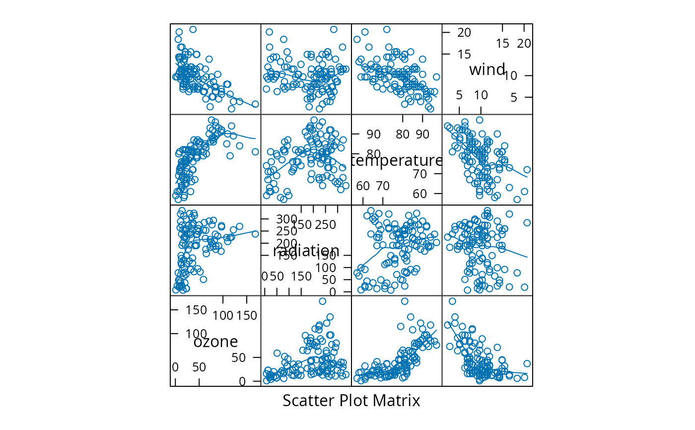
# Scatter plot matrix with loess lines
splom(~environmental,
panel=function(x,y){
panel.xyplot(x,y)
panel.loess(x,y)
}
)
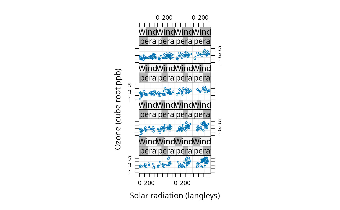
 # Conditioned plot similar to figure 5.3 from Cleveland
attach(environmental)
Temperature <- equal.count(temperature, 4, 1/2)
Wind <- equal.count(wind, 4, 1/2)
xyplot((ozone^(1/3)) ~ radiation | Temperature * Wind,
aspect=1,
prepanel = function(x, y)
prepanel.loess(x, y, span = 1),
panel = function(x, y){
panel.grid(h = 2, v = 2)
panel.xyplot(x, y, cex = .5)
panel.loess(x, y, span = 1)
},
xlab = "Solar radiation (langleys)",
ylab = "Ozone (cube root ppb)")
# Conditioned plot similar to figure 5.3 from Cleveland
attach(environmental)
Temperature <- equal.count(temperature, 4, 1/2)
Wind <- equal.count(wind, 4, 1/2)
xyplot((ozone^(1/3)) ~ radiation | Temperature * Wind,
aspect=1,
prepanel = function(x, y)
prepanel.loess(x, y, span = 1),
panel = function(x, y){
panel.grid(h = 2, v = 2)
panel.xyplot(x, y, cex = .5)
panel.loess(x, y, span = 1)
},
xlab = "Solar radiation (langleys)",
ylab = "Ozone (cube root ppb)")
 detach()
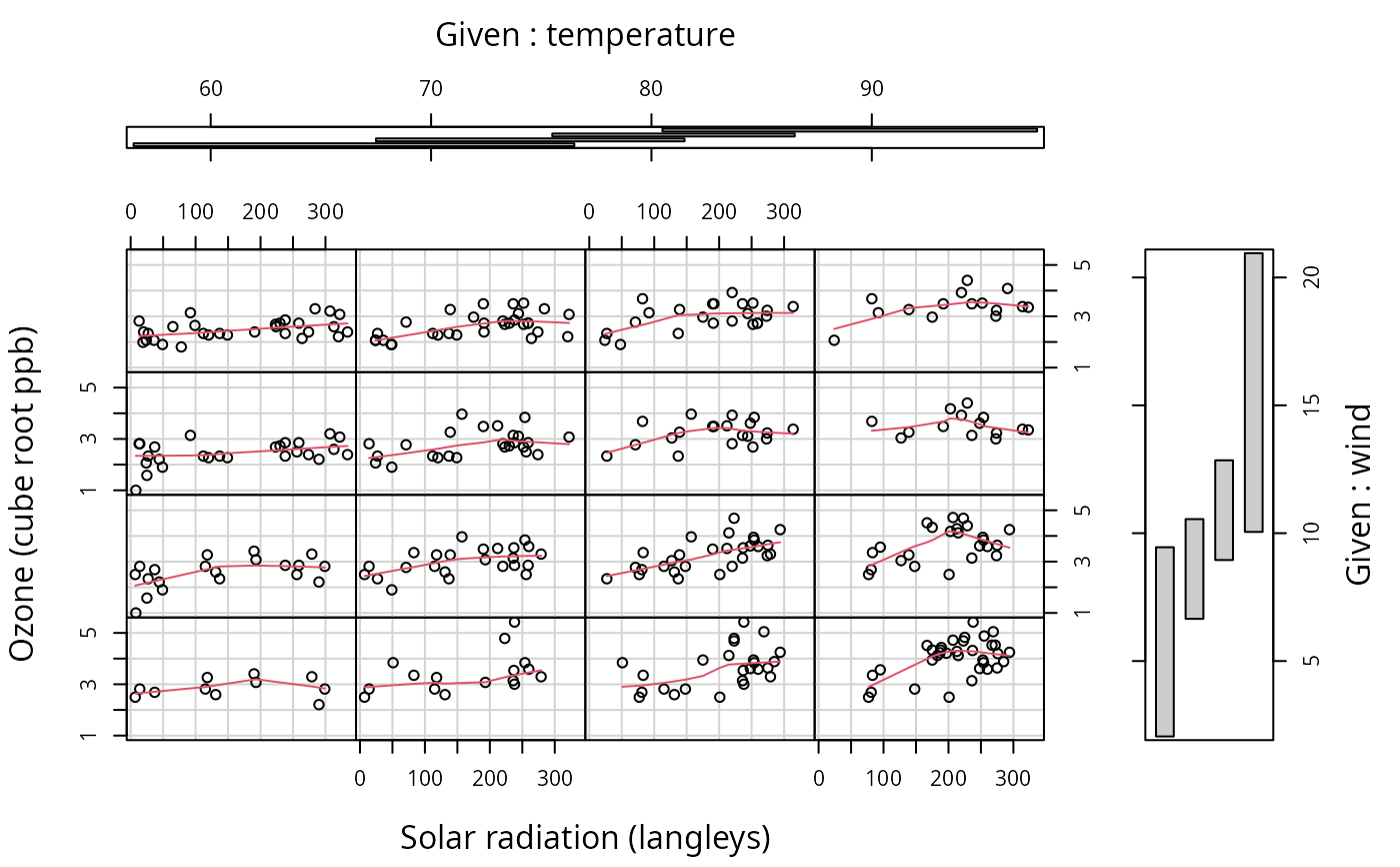
# Similar display using the coplot function
with(environmental,{
coplot((ozone^.33) ~ radiation | temperature * wind,
number=c(4,4),
panel = function(x, y, ...) panel.smooth(x, y, span = .8, ...),
xlab="Solar radiation (langleys)",
ylab="Ozone (cube root ppb)")
})
detach()
# Similar display using the coplot function
with(environmental,{
coplot((ozone^.33) ~ radiation | temperature * wind,
number=c(4,4),
panel = function(x, y, ...) panel.smooth(x, y, span = .8, ...),
xlab="Solar radiation (langleys)",
ylab="Ozone (cube root ppb)")
})