Custom Polynomial Models
‘ggpmisc’ 0.6.2
Pedro J. Aphalo
2025-07-23
Source:vignettes/articles/poly-advanced.Rmd
poly-advanced.RmdAims of ‘ggpmisc’ and caveats
Package ‘ggpmisc’ makes it easier to add to plots created using ‘ggplot2’ annotations based on fitted models and other statistics. It does this by wrapping existing model fit and other functions. The same annotations can be produced by calling the model fit functions, extracting the desired estimates and adding them to plots. There are two advantages in wrapping these functions in an extension to package ‘ggplot2’: 1) we ensure the coupling of graphical elements and the annotations by building all elements of the plot using the same data and a consistent grammar and 2) we make it easier to annotate plots to the casual user of R, already familiar with the grammar of graphics.
To avoid confusion it is good to make clear what may seem obvious to some: if no plot is needed, then there is no reason to use this package. The values shown as annotations are not computed by ‘ggpmisc’ but instead by the usual model-fit and statistical functions from R and other packages. The same is true for model predictions, residuals, etc. that some of the functions in ‘ggpmisc’ display as lines, segments, or other graphical elements.
It is also important to remember that in most cases data analysis including exploratory and other stages should take place before annotated plots for publication are produced. Even though data analysis can benefit from combined numerical and graphical representation of the results, the use I envision for ‘ggpmisc’ is mainly for the production of plots for publication or communication of a completed analysis.
Preliminaries
We load all the packages used in the examples.
Attaching package ‘ggpmisc’ also attaches package ‘ggpp’ as it provides several of the geometries used by default in the statistics described below. Package ‘ggpp’ can be loaded and attached on its own, and has separate documentation.
As we will use text and labels on the plotting area we change the default theme to an uncluttered one.
Fitted models in stat_poly_line() and stat_poly_eq()
Both functions are designed for flexibility while still attempting to keep their implementation and use rather straightforward.
Function stat_poly_eq() requires that the model formula is a regular polynomial (with no missing intermediate power terms), with the exception that the intercept can be missing. Function stat_poly_line() has fewer requirements for the argument passed to formula.
Both statistics: * Accept any R function or its name as argument for method, * as long as fitted model object belongs to classes "lm", "rlm", "lqs", "lts" or "gls", as tested with inherits(), and additionally models of other classes as long as methods are available. * Their implementation tolerates some missing methods and fields in model fit objects and their summary, i.e., returning NA_real_ or empty character strings depending on the case. * The formula used to construct the equation is, whenever possible, extracted from the fitted model object. Only exceptionally, with this approach fails, the formula passed as argument for formula in the call is used with a warning.
This design makes it possible to use as method existing model fit functions that return an object of one of the classes specifically supported, wrapper functions that call such functions, or in some other way return an object of a known class such as "lm" or a class with suitable methods implemented.
To showcase this, I explore the use of contributed and user defined model fit functions through examples. Several of the examples use facets or grouping to demonstrate how the models fitted depend on the data. The approach can be also useful in the absence of facets and/or groups, for example for dynamic reports or dashboards.
Two frequently use model fit functions that return model fit objects that require special handling to extract values are supported in ‘ggpmisc’ by specific statistics: stat_ma_line() and stat_ma_eq() for mayor axis regression with package ‘lmodel2’, and stat_quant_line(), stat_quant_band() and stat_quant_equation() for quantile regression with package ‘quantreg’. Their use is documented in the User Guide and their help pages.
Existing functions
We consider cases in which fitting linear models with ordinary least squares (OLS) as criterion is unsuitable.
In the case of outliers, many methods are available, and each fit function usually also supports several variations within a class of methods. In robust regression the weight of extreme observations in the computation of the penalty function is decreased compared to OLS. The effect of such decrease can be described as weights ranging continuously between 0 and 1, either actually used in the fit algorithm or computed a posteriori by comparison to OLS. In resistant regression, some observations are ignored altogether, which is equivalent to discrete weights taking one of two values, 0 or 1. Even if these approaches work automatically, similarly as when discarding observations manually, it is important to investigate the origin of outliers.
Generalised least squares (GLS) is an extension to OLS that makes it possible to describe how the variance of the response y varies. GLS supports description of heterogeneous variance by means of variance covariates, and correlation structures.
Error in variance (EIV) methods remove the assumption that the values of the covariate x are measured/known without error. It is important here to stress that linear models (LM) do not require us to assume that there is no variation in x, only that we have observed/measured/know these values without error. To apply most of these methods, we need independently obtained information about the size of the measuring errors affecting covariates.
Not exemplified here, major axis regression (MA), is useful when both x and y values are affected to comparable extents by measurement errors. This is typically the case when there is no causal direction between x and y such as in allometric relationships between body parts of the same individual. See stat_ma_line() and stat_ma_eq().
Quantile regression can be thought as similar to both a regression an a box plot. It makes it possible to fit curves that divide the observations in 2D space into quantiles, approximately preserving this split along a fitted curve of y on x. See stat_quant_line(), stat_quant_band() and stat_quant_eq().
As all these methods use different penalty functions when fitting a model to observations, they yield different estimates of parameter values for the same model formula. For several of these methods the approximate solution is obtained using numeral iteration. In these cases, it is important to check whether the solution is stable with different starting points for random number generation.
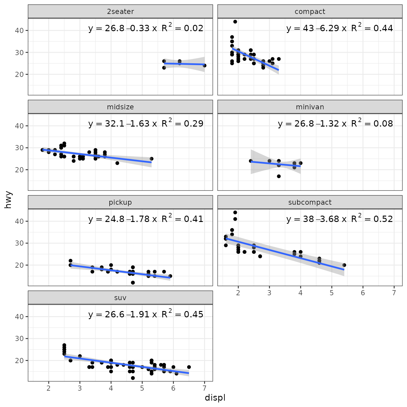
Robust regression (‘MASS’)
Package ‘MASS’ provides function rlm() for “Robust Fitting of Linear Models”. The returned value is an "rlm" object. Class "rlm" is derived from "lm" so the stats work mostly as expected. However, we need to be aware that no or estimates are available and the corresponding labels are empty strings.
ggplot(mpg, aes(displ, hwy)) +
  geom_point() +
  stat_poly_line(method = MASS::rlm) +
  stat_poly_eq(method = MASS::rlm, mapping = use_label("eq", "n"),
               label.x = "right") +
  facet_wrap(~class, ncol = 2)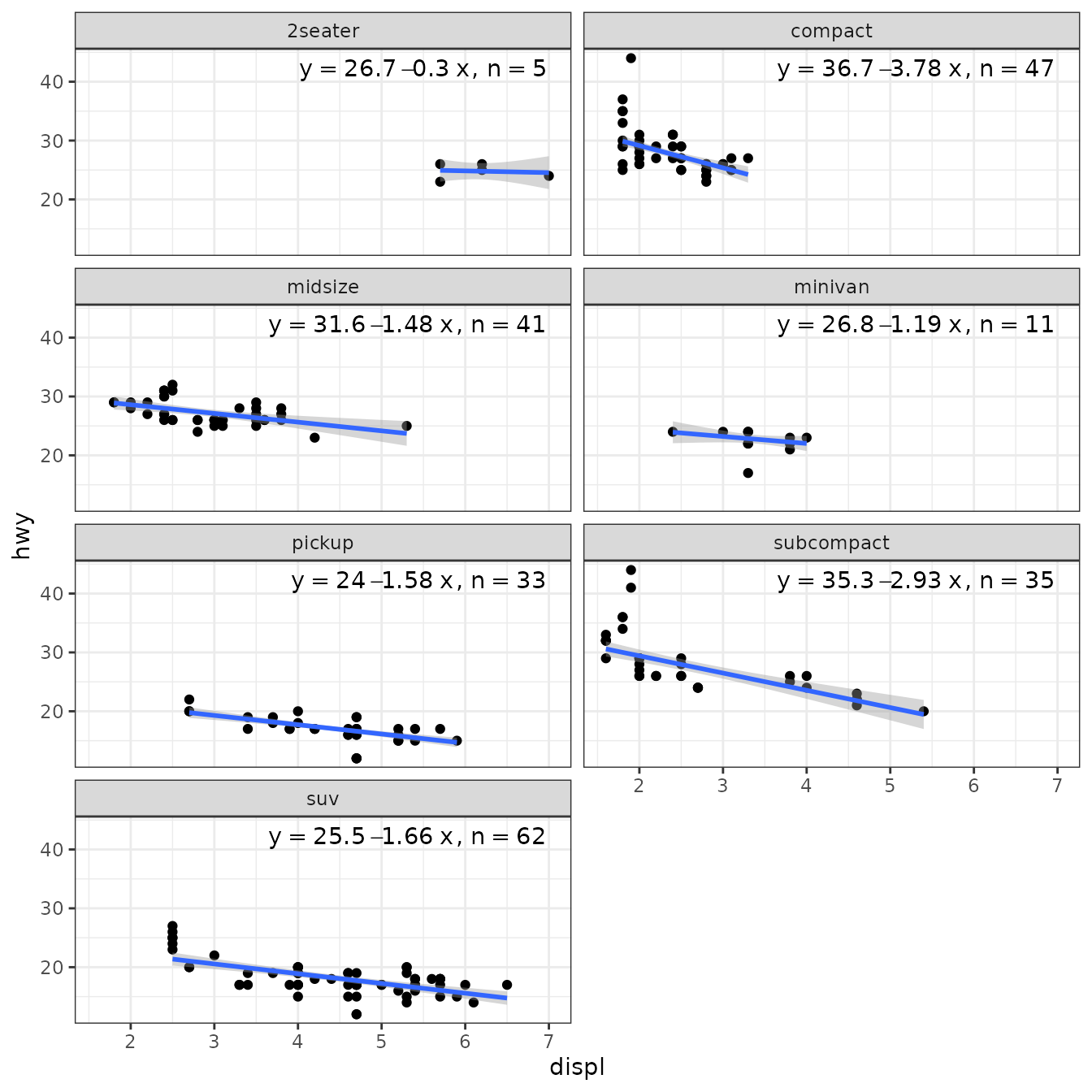
When weights are available, either supplied by the user, or computed as part of the fit, they are returned in data. Having weights available allows encoding them using colour. We here use a robust regression fit with MASS::rlm().
ggplot(mpg, aes(displ, hwy)) +
  stat_poly_eq(use_label("eq", "n", "method"),
               label.x = "right",
               method = MASS::rlm) +
  stat_poly_line(method = MASS::rlm, colour = "black") +
  stat_fit_deviations(method = "rlm",
                      mapping = aes(colour = after_stat(robustness.weights)),
                      show.legend = TRUE,
                      geom = "point") +
  scale_color_gradient(low = "red", high = "blue", limits = c(0, 1)) +
  theme(legend.position = "top")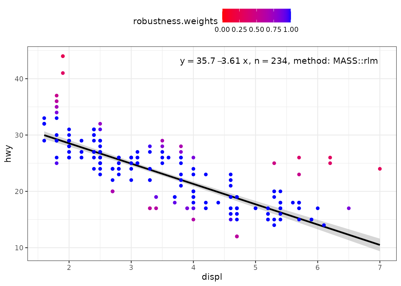
my.formula <- y ~ poly(x, 2, raw = TRUE)
ggplot(mpg, aes(displ, hwy)) +
  stat_poly_eq(use_label("eq", "n", "method"),
               formula = my.formula,
               label.x = "right",
               method = MASS::rlm) +
  stat_poly_line(method = MASS::rlm,
                 formula = my.formula,
                 colour = "black") +
  stat_fit_deviations(mapping = aes(colour = after_stat(robustness.weights)),
                      method = "rlm",
                      formula = my.formula,
                      show.legend = TRUE,
                      geom = "point") +
  scale_color_gradient(low = "red", high = "blue", limits = c(0, 1)) +
  theme(legend.position = "top")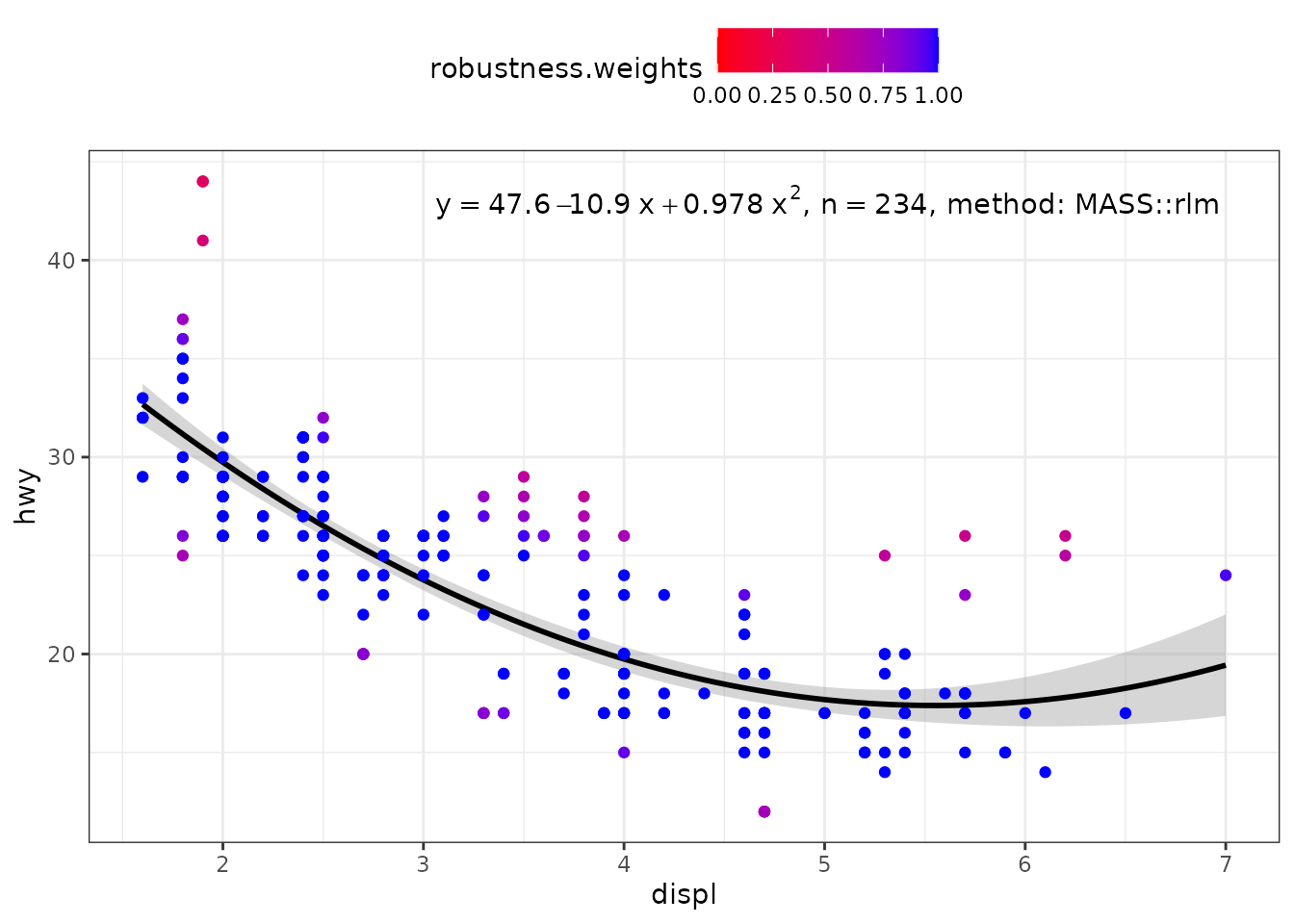
Robust regression (‘robustbase’)
Package ‘robustbase’ provides function lmrob() for “MM-type Estimators for Linear Regression”. The returned value is an "lmrob" object. Class "lmrob" is derived from "lm" so the stats work mostly as expected. However, we need to be aware that no or estimates are available and the corresponding labels are empty strings.
ggplot(mpg, aes(displ, hwy)) +
  geom_point() +
  stat_poly_line(method = robustbase::lmrob) +
  stat_poly_eq(method = robustbase::lmrob, mapping = use_label("eq", "R2"),
               label.x = "right") +
  theme(legend.position = "bottom") +
  facet_wrap(~class, ncol = 2)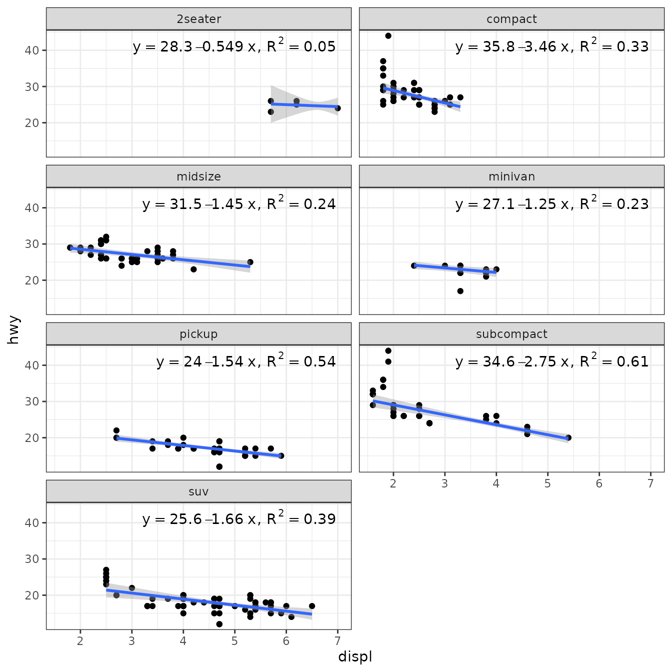
When weights are available, either supplied by the user, or computed as part of the fit, they are returned in data. Having weights available allows encoding them using colour. We here use a robust regression fit with MASS::rlm().
ggplot(mpg, aes(displ, hwy)) +
  stat_poly_eq(use_label("eq", "R2", "method"),
               label.x = "right",
               method = robustbase::lmrob) +
  stat_poly_line(method = robustbase::lmrob, colour = "black") +
  stat_fit_deviations(method = robustbase::lmrob,
                      mapping = aes(colour = after_stat(robustness.weights)),
                      show.legend = TRUE,
                      geom = "point") +
  scale_color_gradient(name = "Robustness weights",
                       low = "red", high = "blue", limits = c(0, 1)) +
  theme(legend.position = "top")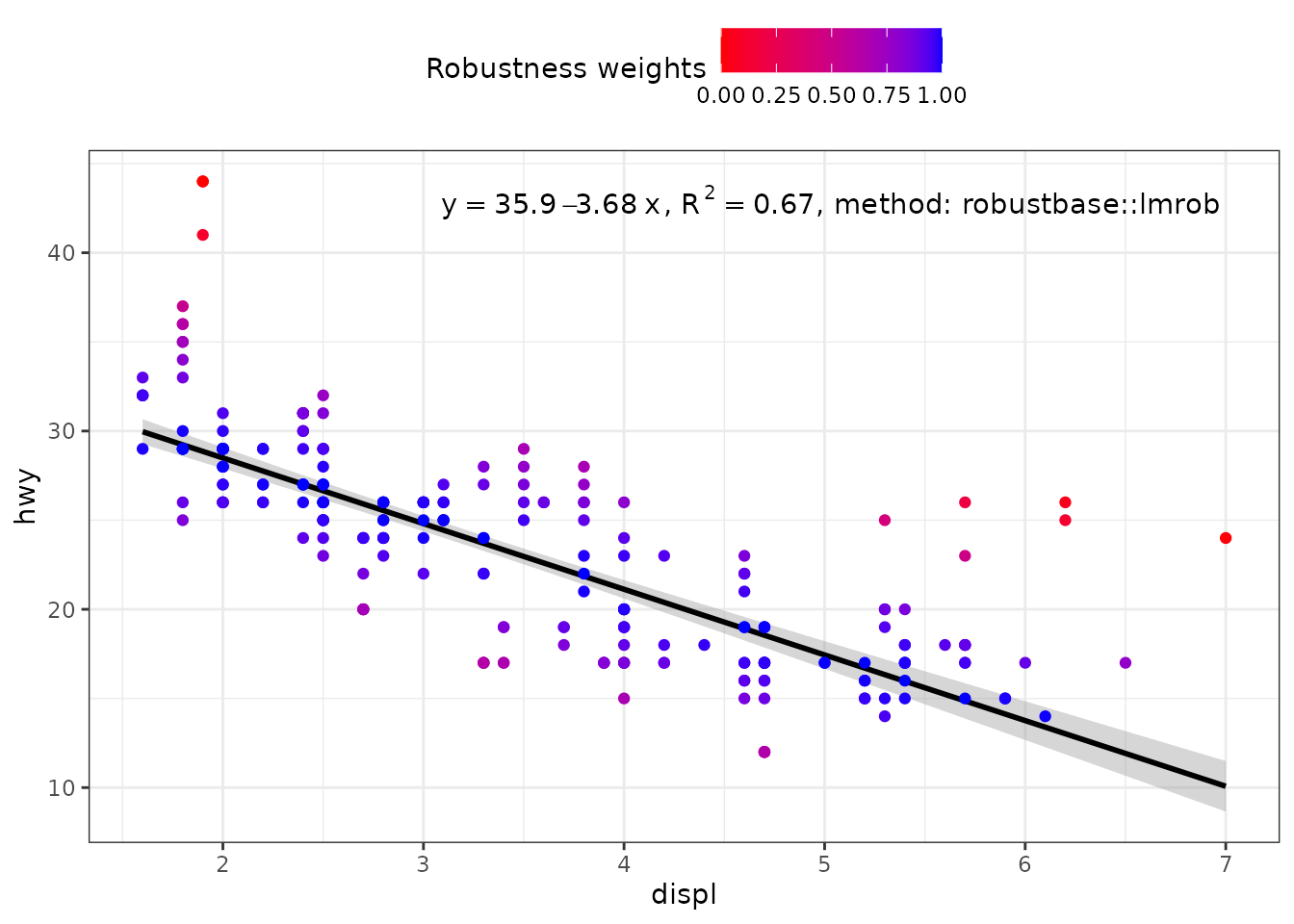
my.formula <- y ~ poly(x, 2, raw = TRUE)
ggplot(mpg, aes(displ, hwy)) +
  stat_poly_eq(use_label("eq", "R2", "method"),
               formula = my.formula,
               label.x = "right",
               method = robustbase::lmrob) +
  stat_poly_line(method = robustbase::lmrob,
                 formula = my.formula,
                 colour = "black") +
  stat_fit_deviations(method = robustbase::lmrob,
                      mapping = aes(colour = after_stat(robustness.weights)),
                      formula = my.formula,
                      show.legend = TRUE,
                      geom = "point") +
  scale_color_gradient(name = "Robustness weights",
                       low = "red", high = "blue", limits = c(0, 1)) +
  theme(legend.position = "top")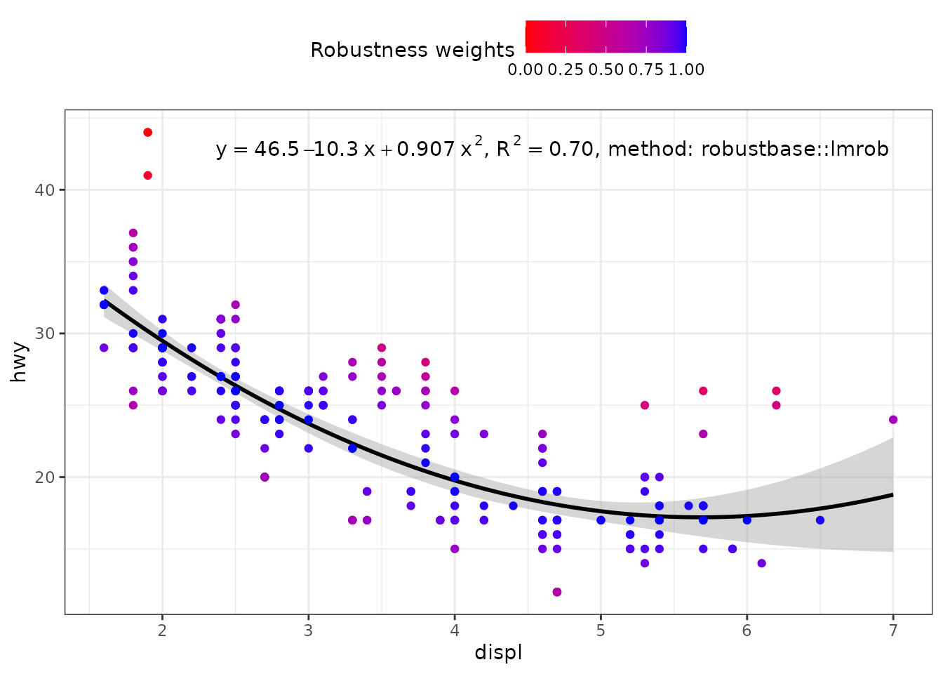
Resistant regression (‘MASS’)
Package ‘MASS’ provides function lqs() for “Resistant Regression”. The returned value is an "lqs" object. Class "rlm" is not derived from "lm" but the structure is similar. However, we need to be aware that no or estimates are available and the corresponding labels are empty strings.
ggplot(mpg, aes(displ, hwy)) +
  geom_point() +
  stat_poly_line(method = MASS::lqs, se = FALSE) +
  stat_poly_eq(method = MASS::lqs, mapping = use_label("eq", "n"),
               label.x = "right") +
  theme(legend.position = "bottom") +
  facet_wrap(~class, ncol = 2)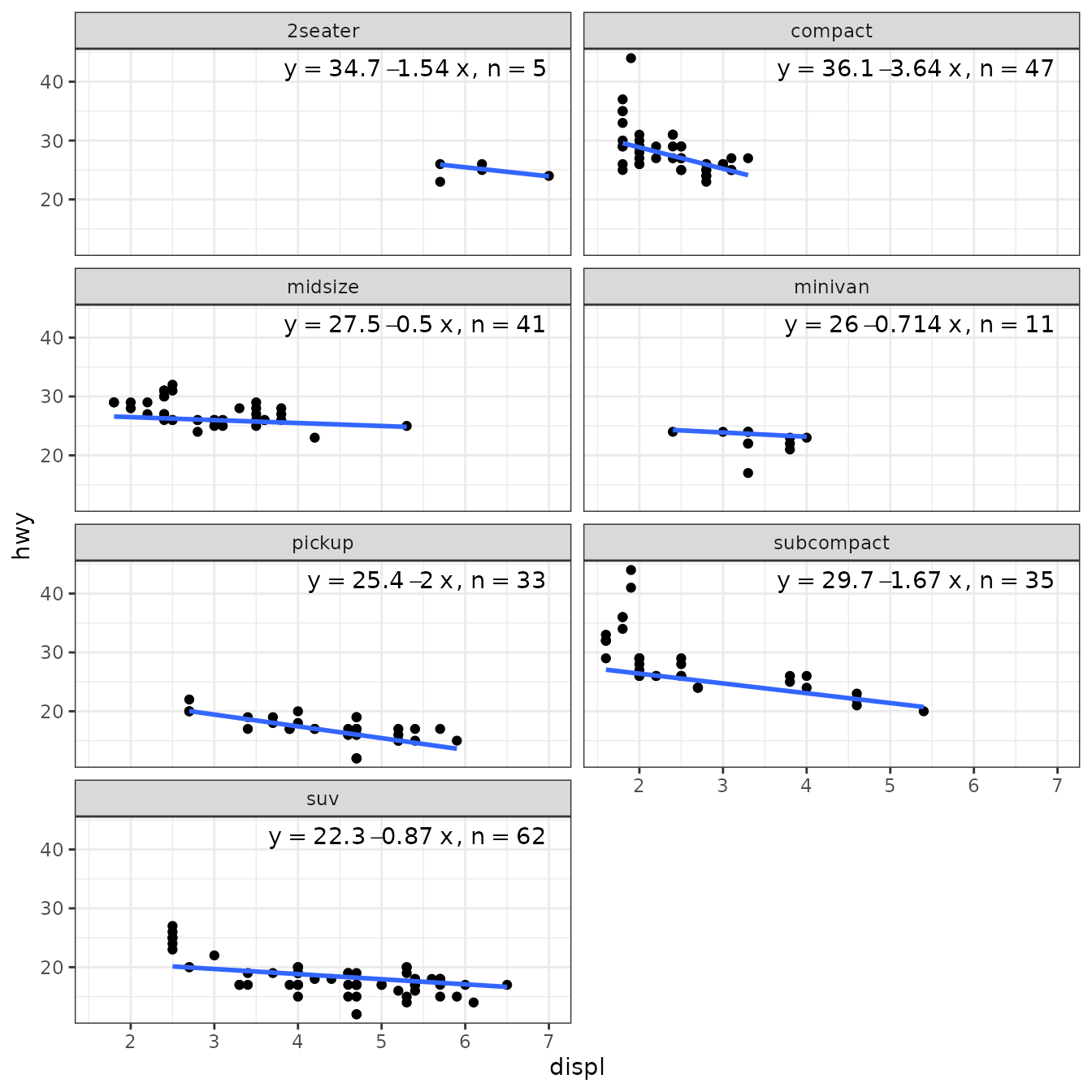
Weights are currently not available for MASS::lqs() and NA vectors are returned instead. To highlight the LTS weights, rosbustbase::ltsReg() can be used as shown in the next section.
ggplot(mpg, aes(displ, hwy)) +
  stat_poly_eq(use_label("eq", "n", "method"),
               label.x = "right",
               method = MASS::lqs) +
  stat_poly_line(method = "lqs:lms", colour = "black") +
  stat_fit_deviations(method = MASS::lqs,
                      mapping =
                        aes(colour = factor(after_stat(robustness.weights))),
                      show.legend = TRUE,
                      geom = "point") +
  scale_color_manual(name = "LTS weights",
                     values = c("0" = "red", "1" = "black")) +
  theme(legend.position = "top")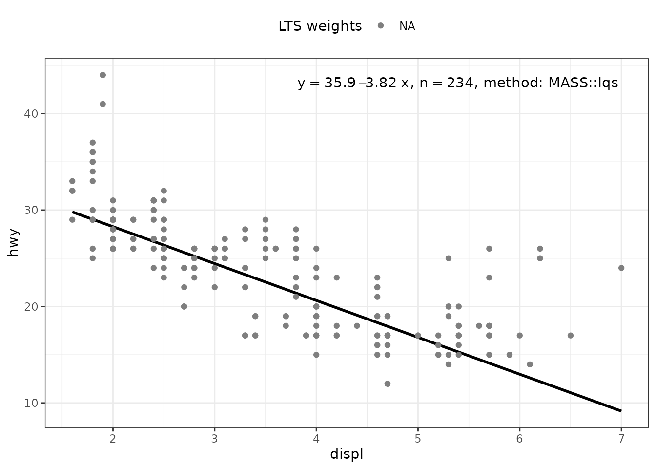
my.formula <- y ~ poly(x, 2, raw = TRUE)
ggplot(mpg, aes(displ, hwy)) +
  stat_poly_eq(use_label("eq", "n", "method"),
               formula = my.formula,
               label.x = "right",
               method = MASS::lqs) +
  stat_poly_line(method = "lqs:lms",
                 formula = my.formula,
                 colour = "black") +
  stat_fit_deviations(mapping =
                        aes(colour = factor(after_stat(robustness.weights))),
                      method = MASS::lqs,
                      formula = my.formula,
                      show.legend = TRUE,
                      geom = "point") +
  scale_color_manual(name = "LTS weights",
                     values = c("0" = "red", "1" = "black")) +
  theme(legend.position = "top")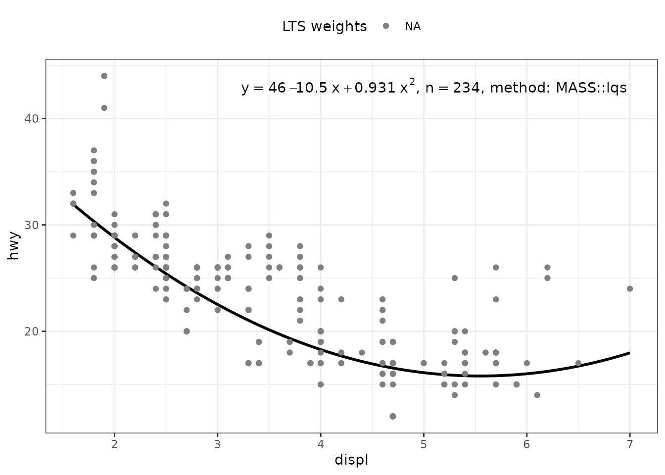
Resistant regression (‘robustbase’)
Package ‘robustbase’ provides function ltsReg() for “least trimmed squares” regression. The returned value is an "lts" object. The usual accessors functions are available for Class "lts".
ggplot(mpg, aes(displ, hwy)) +
  geom_point() +
  stat_poly_line(method = robustbase::ltsReg, se = FALSE) +
  stat_poly_eq(method = robustbase::ltsReg, mapping = use_label("eq", "n"),
               label.x = "right") +
  theme(legend.position = "bottom") +
  facet_wrap(~class, ncol = 2)
#> Fitted values returned
#> Fitted values returned
#> Fitted values returned
#> Fitted values returned
#> Fitted values returned
#> Fitted values returned
#> Fitted values returned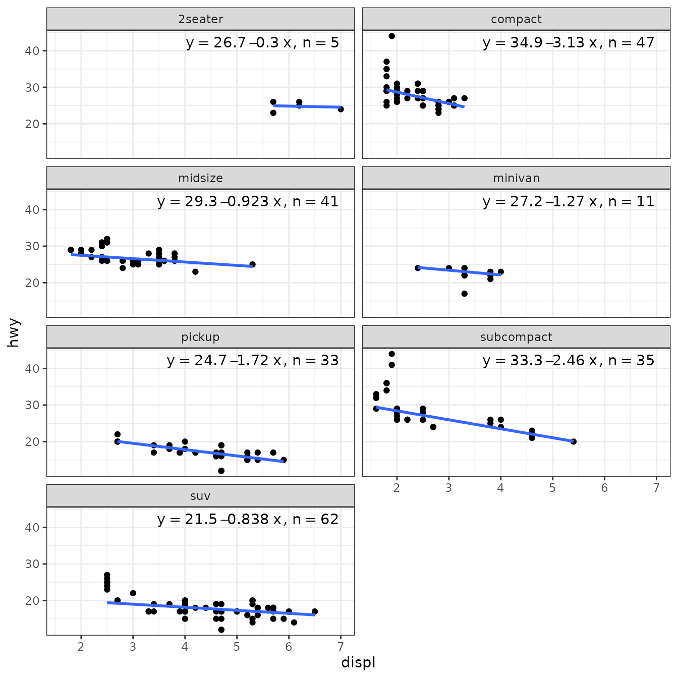
If no predict() method is found for a model fit object, stat_poly_line() searches for method fitted(), which is nearly always available. This is how the "lts" objects returned by robustbase::ltsReg() are by default supported.
For a linear regression, unless extrapolation is attempted this makes little, if any, difference to the line but no confidence band is displayed. With higher degree polynomials and sparse data this approach can result in a curve that is not smooth. It is possible for users to define the missing specialization for the predict() method. Predicting the fitted line using coefficients() and the known formula is straightforward, while estimating a prediction confidence band can be more difficult.
ggplot(mpg, aes(displ, hwy)) +
  stat_poly_eq(use_label("eq", "R2", "method"),
               label.x = "right",
               method = robustbase::ltsReg) +
  stat_poly_line(method = robustbase::ltsReg, colour = "black") +
  stat_fit_deviations(mapping = aes(colour = factor(after_stat(robustness.weights))),
                      geom = "point",
                      method = robustbase::ltsReg,
                      show.legend = TRUE) +
  scale_color_manual(name = "LTS weights",
                     values = c("0" = "red", "1" = "blue")) +
  theme(legend.position = "top")
#> Fitted values returned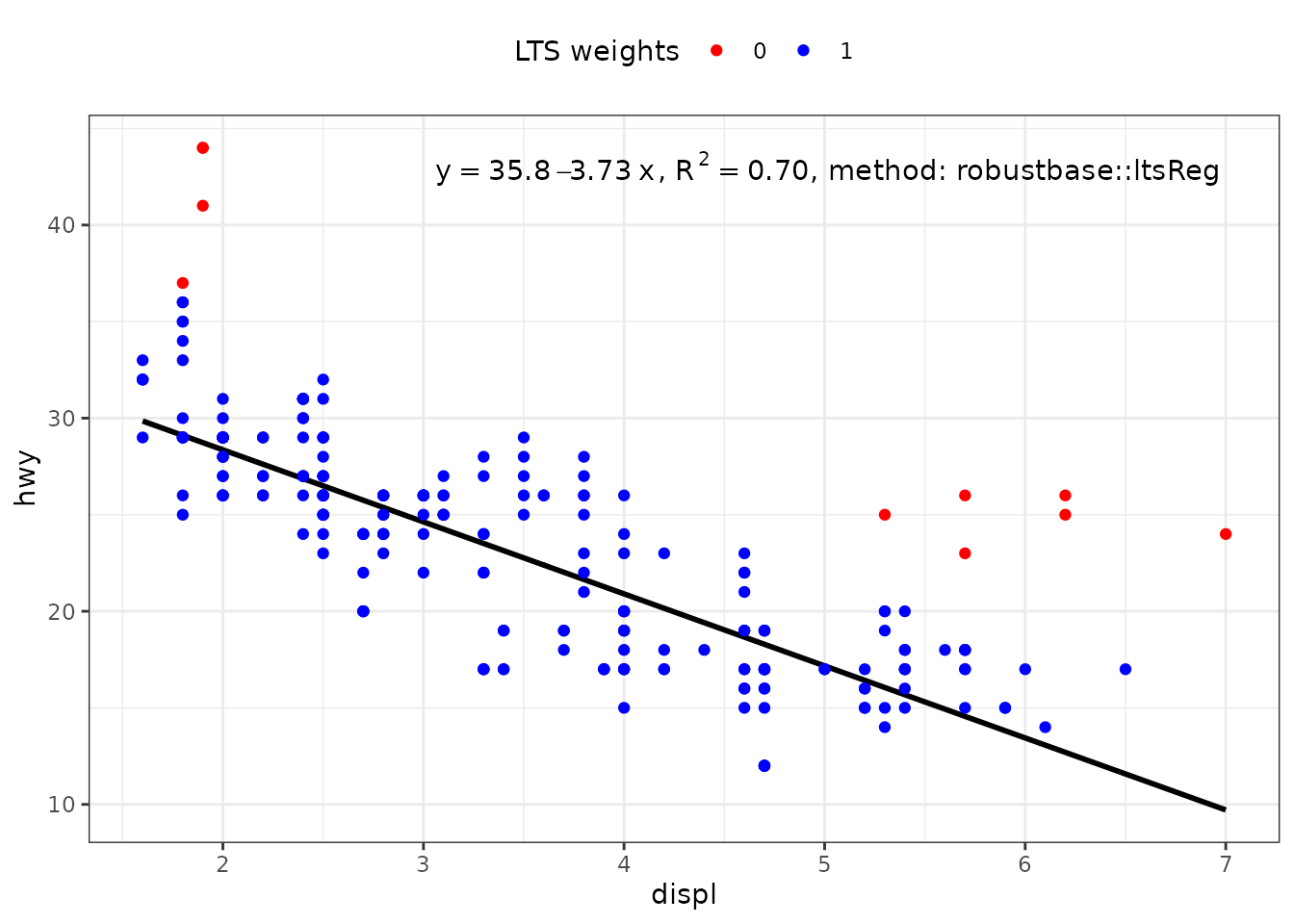
my.formula <- y ~ poly(x, 2, raw = TRUE)
ggplot(mpg, aes(displ, hwy)) +
  stat_poly_eq(use_label("eq", "R2", "method"),
               label.x = "right",
               formula = my.formula,
               method = robustbase::ltsReg) +
  stat_poly_line(method = robustbase::ltsReg,
                 formula = my.formula,
                 colour = "black") +
  stat_fit_deviations(mapping = aes(colour = factor(after_stat(robustness.weights))),
                      formula = my.formula,
                      geom = "point",
                      method = robustbase::ltsReg,
                      show.legend = TRUE) +
  scale_color_manual(name = "LTS weights",
                     values = c("0" = "red", "1" = "blue")) +
  theme(legend.position = "top")
#> Fitted values returned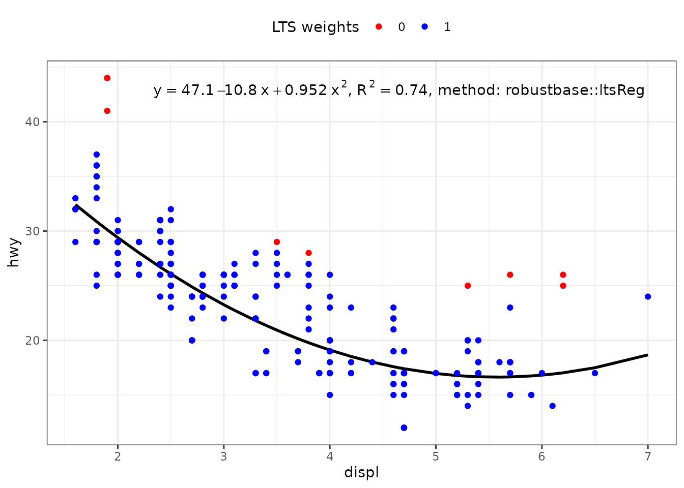
Generalized Least Squares (‘nlme’)
In ‘ggpmisc’ (>= 0.6.2) function gls() from package ‘nlme’ is supported natively by functions stat_poly_line() and stat_poly_eq(). In this example, using a variance covariate, the computations do not converge with the data in one of the plot panels.
ggplot(mpg, aes(displ, hwy)) +
   geom_point() +
   stat_poly_line(method = gls,
                  method.args = list(weights = varPower()),
                  se = FALSE) +
   stat_poly_eq(method = gls,
                method.args = list(weights = varPower()),
                mapping = use_label("eq"),
   label.x = "right") +
   theme(legend.position = "bottom") +
   facet_wrap(~class, ncol = 2)
#> Warning: Computation failed in `stat_poly_line()`.
#> Caused by error:
#> ! maximum number of iterations reached without convergence
#> Warning: Computation failed in `stat_poly_eq()`.
#> Caused by error:
#> ! maximum number of iterations reached without convergence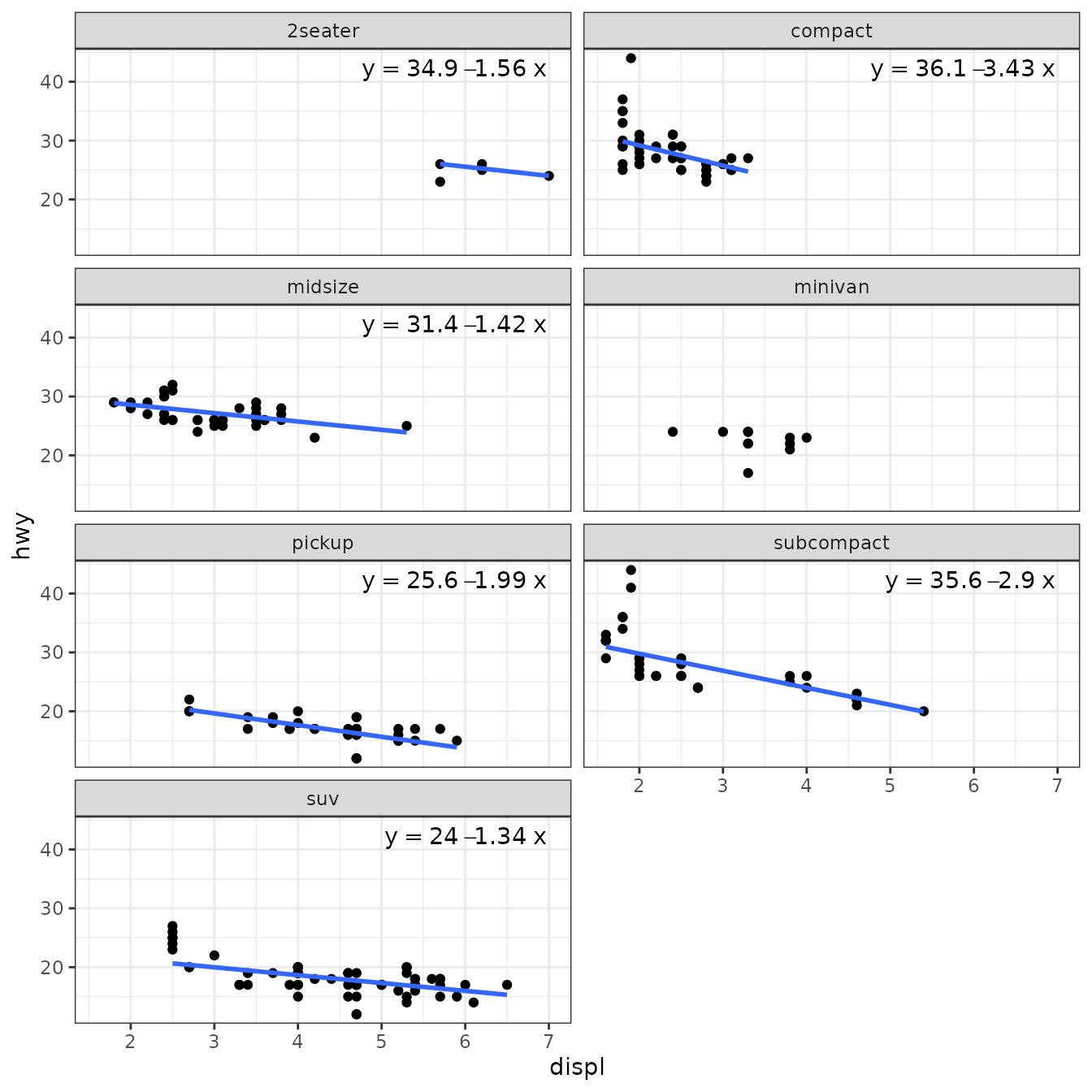
User defined functions
As mentioned above, layer functions stat_poly_line() and stat_poly_eq() support the use of several different model fit functions, as long as the estimates and predictions can be extracted. In the case of stat_poly_eq(), the model formula embedded in this object must be a polynomial. The variables mapped to x and y aesthetics must be continuous numeric, times or dates. Models are fitted separately to each group and plot panel, similarly as by ggplot2::stat_smooth(). ‘ggpmisc’ provides additional flexibility by delaying some decisions until after the models have been fit to the observations.
stat_poly_line() and stat_poly_eq() adjust their behaviour based on the class of the model object returned by the method, not the name of the method passed in the call as argument. Thus, the class of the model fit object returned can vary in response to data, and thus also be different for different panels or groups in the same plot.
stat_poly_eq() builds the fitted model equation based on the model formula extracted from the model fit object, which can differ from that passed as argument to formula when calling the statistic. Thus, the model formula returned by the function passed as argument for method vary by group and/or panel.As the examples below demonstrate, this approach can be very useful. In addition, NA can be used to signal to stat_poly_line() and stat_poly_eq() that no model has been fit for a group or panel.
Below I use lm() and "lm" model fit objects in most examples, but the same approaches can be applied to objects of other classes, including "rlm", "lmrob", ’“lqs”,“lts”,“gls”`.
Fit or not
In the first example we fit a model only if a minimum number of distinct x values are present in data. We define a function that instead of fitting the model, returns NA when the condition is not fulfilled. Here "x" is the aesthetic, and has to be replaced by "y" depending on orientation.
fit_or_not <- function(formula, data, ..., orientation = "x") {
  if (length(unique(data[[orientation]])) > 5) {
    lm(formula = formula, data = data, ...)
  } else {
    NA_real_
  }
}
Instead of using stats::lm() as method, we pass our wrapper function fit_or_not() as the method. As the function returns either an "lm" object from the wrapped call to lm() or NA, the call to the statistics can make use of all other features as needed.
ggplot(mpg, aes(displ, hwy)) +
  geom_point() +
  stat_poly_line(method = "fit_or_not") +
  stat_poly_eq(method = fit_or_not,
               mapping = use_label("eq", "R2"),
               label.x = "right") +
  stat_panel_counts(label.x = "left", label.y = "bottom") +
  theme(legend.position = "bottom") +
  facet_wrap(~class, ncol = 2)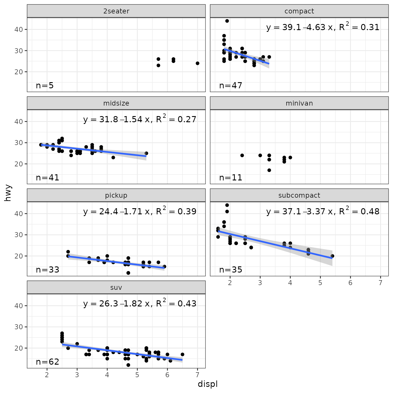
Degree of polynomial
Not fitting a model, is a drastic solution. An alternative that we implement next, is to plot the mean when the slope of the linear regression is not significantly different from zero. In the example below instead of using stats::lm() as method, we define a different wrapper function that tests for the significance of the slope in linear regression, and if not significant, fits the mean instead. _This works because the model formula is extracted from the fitted model rather than using the argument passed by the user in the call to the statistics.
Fitting different models to different panels is supported. User-defined method functions are required to return an object that inherits from class "lm". The function is applied per group and panel, and the model formula fitted can differ among them, as it is retrieved from this object to construct the equation label.
In the example below instead of using stats::lm() as method, we define a wrapper function that tests for the significance of the slope in linear regression, and if not significant, fits the mean instead.
poly_or_mean <- function(formula, data, ...) {
   fm <- lm(formula = formula, data = data, ...)
   if (anova(fm)[["Pr(>F)"]][1] > 0.1) {
      lm(formula = y ~ 1, data = data, ...)
   } else {
      fm
   }
}
We then use our function poly_or_mean() as the method.
ggplot(mpg, aes(displ, hwy)) +
   geom_point() +
   stat_poly_line(method = "poly_or_mean") +
   stat_poly_eq(method = poly_or_mean,
               mapping = use_label("eq", "R2"),
               label.x = "right") +
   theme(legend.position = "bottom") +
   facet_wrap(~class, ncol = 2)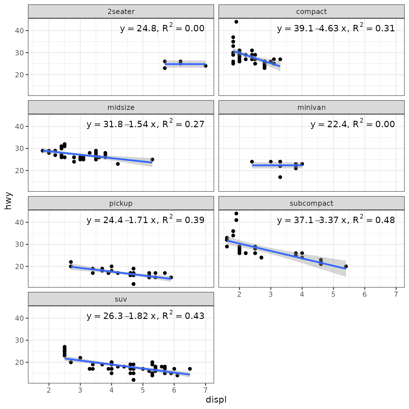
ggplot(mpg, aes(displ, hwy, color = class)) +
   geom_point() +
   stat_poly_line(method = "poly_or_mean") +
   stat_poly_eq(method = poly_or_mean,
               mapping = use_label("eq"),
               label.x = "right") +
   theme(legend.position = "top")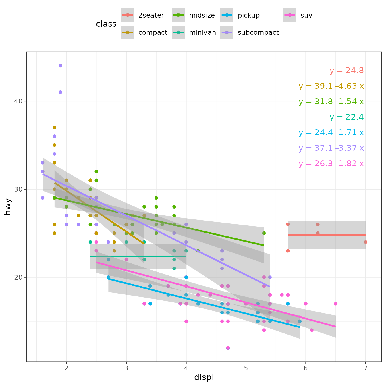
A different approach to selecting the degree of a polynomial is to use stepwise selection based on AIC. In this case the formula passed as argument is the “upper” degree of the polynomial. All lower degree polynomials are fitted and the one with lowest AIC used.
best_poly_lm <- function(formula, data, ...) {
  poly.term <- as.character(formula)[3]
  degree <- as.numeric(gsub("poly[(]x, |, raw = TRUE|[)]", "", poly.term))
  fms <- list()
  AICs <- numeric(degree)
  for (d in 1:degree) {
    # we need to define the formula with the value of degree replaced
    working.formula <- as.formula(bquote(y ~ poly(x, degree = .(d), raw = TRUE)))
    fms[[d]] <- lm(formula = working.formula, data = data, ...)
    AICs[d] <- AIC(fms[[d]])
  }
  fms[[which.min(AICs)[1]]] # if there is a tie, we take the simplest
}
We then use our function best_poly_lm() as the method.
ggplot(mpg, aes(displ, hwy)) +
  geom_point() +
  stat_poly_line(formula = y ~ poly(x, 3, raw = TRUE), method = "best_poly_lm") +
  stat_poly_eq(formula = y ~ poly(x, 3, raw = TRUE), method = "best_poly_lm",
               mapping = use_label("eq", "AIC"),
               size = 2.8,
               label.x = "right") +
  expand_limits(y = c(0, 65)) +
  facet_wrap(~class, ncol = 2)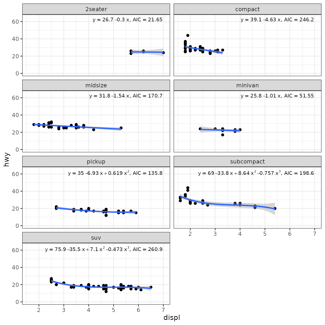
ggplot(mpg, aes(displ, hwy, color = class)) +
  geom_point() +
  stat_poly_line(formula = y ~ poly(x, 3, raw = TRUE), method = "best_poly_lm") +
  stat_poly_eq(formula = y ~ poly(x, 3, raw = TRUE), method = "best_poly_lm",
               mapping = use_label("eq", "AIC"),
               label.x = "right") +
  expand_limits(y = c(0, 65)) +
  theme(legend.position = "top")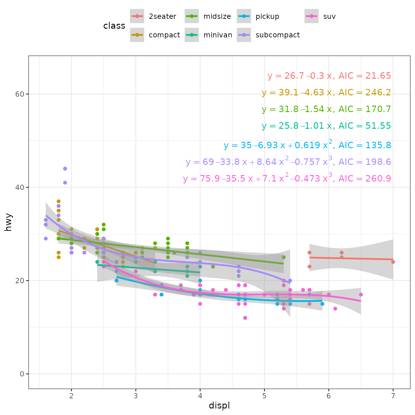
Work-arounds
Some model fit functions return object for which no predict() method exist. In such cases, as users we can define such a method. More difficult situations can be faced. In this last section I show a situation I faced when trying to use package ‘refitME’. The functions exported by this package fail when called from within a function, so they do not currently work if passed as an argument for method. Below, a temporary work-around based on a solution provided by the maintainer of ‘refitME’ is shown.
Errors in variables (‘refitME’)
As ‘refitME’ functions return a model fit object of the same class as that received as input, a model fitted with lm() could be, in principle, refit in a user-defined wrapper function as those above, calling first lm() and re-fitting the obtained model with a refitME::refitME() as shown in the code chunk below. However, at the moment the functions in package ‘refitME’ fail when called from within another function.
lm_EIV <- function(formula, data, ..., sigma.sq.u) {
  fm <- lm(formula = formula, data = data, ...)
  MCEMfit_glm(mod = fm, family = "gaussian", sigma.sq.u = sigma.sq.u)
}
After defining such a function, we could then use our function lm_EIV() as the method.
ggplot(mpg, aes(displ, hwy)) +
   geom_point() +
   stat_poly_line(method = "lm_EIV", method.args = c(sigma.sq.u = 0)) +
   stat_poly_eq(method = "lm_EIV", method.args = c(sigma.sq.u = 0),
                mapping = use_label("eq"),
   label.x = "right") +
   theme(legend.position = "bottom") +
   facet_wrap(~class, ncol = 2)
Produces one warning like below for each call of the statistics.
Warning: Computation failed in `stat_poly_eq()`.
Caused by error in `names(new.dat)[c(1, which(names(mod$data) %in% names.w))] <- names(mod$data)[c(1, which(names(mod$data) %in% names.w))]`:
! replacement has length zero```
I have reported the problem through a GitHub issue to Jakub Stoklosa, the maintainer of ‘refitME’, and he is looking for a permanent solution. Meanwhile, he has provided a temporary fix that I copy below with a few small edits to the ggplot code. Many thanks to Jakub Stoklosa for his very fast answer!
rm(list = ls(pattern = "*"))

library(ggplot2)
library(ggpmisc)
library(refitME)

lm_EIV <- function(formula, data, ..., sigma.sq.u) {
  assign("my.data", value = data, envir = globalenv())
  fm <- lm(formula = formula, data = my.data, ...)
  fit <- refitME(fm, sigma.sq.u)

  fit$coefficients <- Re(fit$coefficients)
  fit$fitted.values <- Re(fit$fitted.values)
  fit$residuals <- Re(fit$residuals)
  fit$effects <- Re(fit$effects)
  fit$linear.predictors <- Re(fit$linear.predictors)
  fit$se <- Re(fit$se)

  if ("qr" %in% names(fit)) {
  fit$qr$qr <- Re(fit$qr$qr)
  fit$qr$qraux <- Re(fit$qr$qraux)
  }

  class(fit) <- c("lm_EIV", "lm")
  return(fit)
}

predict.lm_EIV <- function(object, newdata = NULL, ...) {
  preds <- NextMethod("predict", object, newdata = newdata, ...)

  if (is.numeric(preds)) {
    return(Re(preds))
  } else if (is.matrix(preds)) {
    return(Re(preds))
  } else {
    return(preds) # Leave unchanged if not numeric/matrix
  }
}
Here the limitation of ‘ggplot2’ and ‘ggpmisc’ in that the fit is recomputed in each layer causes a further difficulty, as with most algorithms using random numbers, the successive refits do not necessarily produce the exact same results. In this case, the equation and line are not matched, and the mismatch can be large for large values of sigma.sq.u and low replication, especially in the presence of outliers.
This is something that can most likely be fixed in ‘ggpmisc’ by setting the seed of the RNG. To check that work-around is working as expected, we set sigma.sq.u = 0 effectively using an OLS approach and expecting values nearly identical as with lm().
ggplot(mpg, aes(x = displ, y = hwy)) +
  geom_point() +
  stat_poly_line(aes(y = hwy),
                 method = "lm_EIV",
                 method.args = list(sigma.sq.u = 0)) +
  stat_poly_eq(aes(y = hwy,
                   label = paste(after_stat(eq.label), after_stat(rr.label),
                                 sep = "~~")),
               method = "lm_EIV",
               method.args = list(sigma.sq.u = 0),
               label.x = "right") +
  facet_wrap(~class, ncol = 2)
#> [1] 2
#> [1] 2
#> [1] 2
#> [1] 2
#> [1] 2
#> [1] 2
#> [1] 2
#> [1] 2
#> [1] 2
#> [1] 2
#> [1] 2
#> [1] 2
#> [1] 2
#> [1] 2
We do not know the measurement error for the measurement of displ, the displacement volume of the engines. For this example we make up a value: sigma.sq.u = 0.01 expecting estimates different from above and with lm().
ggplot(mpg, aes(x = displ, y = hwy)) +
  geom_point() +
  stat_poly_line(aes(y = hwy),
                 method = "lm_EIV",
                 method.args = list(sigma.sq.u = 0.01)) +
  stat_poly_eq(aes(y = hwy,
                   label = paste(after_stat(eq.label), after_stat(rr.label),
                                 sep = "~~")),
               method = "lm_EIV",
               method.args = list(sigma.sq.u = 0.01),
               label.x = "right") +
  facet_wrap(~class, ncol = 2)
#> [1] 5
#> [1] 11
#> [1] 6
#> [1] 7
#> [1] 6
#> [1] 9
#> [1] 6
#> [1] 5
#> [1] 10
#> [1] 6
#> [1] 6
#> [1] 6
#> [1] 8
#> [1] 6