Equation, p-value, \(R^2\), AIC and BIC of fitted polynomial

stat_poly_eq fits a polynomial, by default with stats::lm(), but alternatively using robust regression or generalized least squares. Using the fitted model it generates several labels including the fitted model equation, p-value, F-value, coefficient of determination (R^2), 'AIC', 'BIC', number of observations and method name, if available.

stat_poly_eq(
  mapping = NULL,
  data = NULL,
  geom = "text_npc",
  position = "identity",
  ...,
  formula = NULL,
  method = "lm",
  method.args = list(),
  n.min = 2L,
  eq.with.lhs = TRUE,
  eq.x.rhs = NULL,
  small.r = getOption("ggpmisc.small.r", default = FALSE),
  small.p = getOption("ggpmisc.small.p", default = FALSE),
  CI.brackets = c("[", "]"),
  rsquared.conf.level = 0.95,
  coef.digits = 3,
  coef.keep.zeros = TRUE,
  decreasing = getOption("ggpmisc.decreasing.poly.eq", FALSE),
  rr.digits = 2,
  f.digits = 3,
  p.digits = 3,
  label.x = "left",
  label.y = "top",
  hstep = 0,
  vstep = NULL,
  output.type = NULL,
  na.rm = FALSE,
  orientation = NA,
  parse = NULL,
  show.legend = FALSE,
  inherit.aes = TRUE
)

Arguments

mapping: The aesthetic mapping, usually constructed with aes. Only needs to be set at the layer level if you are overriding the plot defaults.
data: A layer specific dataset, only needed if you want to override the plot defaults.
geom: The geometric object to use display the data
position: The position adjustment to use for overlapping points on this layer
...: other arguments passed on to layer. This can include aesthetics whose values you want to set, not map. See layer for more details.
formula: a formula object. Using aesthetic names x and y instead of original variable names.
method: function or character If character, "lm", "rlm", "lqs". "gls" or the name of a model fit function are accepted, possibly followed by the fit function's method argument separated by a colon (e.g. "rlm:M"). If a function is different to lm(), rlm(), lqs() or gls(), it must have formal parameters named formula, data, weights, and method, and return a model fit object of class "lm", class "lqs" or class "gls".
method.args: named list with additional arguments.
n.min: integer Minimum number of distinct values in the explanatory variable (on the rhs of formula) for fitting to the attempted.
eq.with.lhs: If character the string is pasted to the front of the equation label before parsing or a logical (see note).
eq.x.rhs: character this string will be used as replacement for "x" in the model equation when generating the label before parsing it.
small.r, small.p: logical Flags to switch use of lower case r and p for coefficient of determination and p-value.
CI.brackets: character vector of length 2. The opening and closing brackets used for the CI label.
rsquared.conf.level: numeric Confidence level for the returned confidence interval. Set to NA to skip CI computation.
coef.digits, f.digits: integer Number of significant digits to use for the fitted coefficients and F-value.
coef.keep.zeros: logical Keep or drop trailing zeros when formatting the fitted coefficients and F-value.
decreasing: logical It specifies the order of the terms in the returned character string; in increasing (default) or decreasing powers.
rr.digits, p.digits: integer Number of digits after the decimal point to use for \(R^2\) and P-value in labels. If Inf, use exponential notation with three decimal places.
label.x, label.y: numeric with range 0..1 "normalized parent coordinates" (npc units) or character if using geom_text_npc() or geom_label_npc(). If using geom_text() or geom_label() numeric in native data units. If too short they will be recycled.
hstep, vstep: numeric in npc units, the horizontal and vertical step used between labels for different groups.
output.type: character One of "expression", "LaTeX", "text", "markdown" or "numeric".
na.rm: a logical indicating whether NA values should be stripped before the computation proceeds.
orientation: character Either "x" or "y" controlling the default for formula.
parse: logical Passed to the geom. If TRUE, the labels will be parsed into expressions and displayed as described in ?plotmath. Default is TRUE if output.type = "expression" and FALSE otherwise.
show.legend: logical. Should this layer be included in the legends? NA, the default, includes if any aesthetics are mapped. FALSE never includes, and TRUE always includes.
inherit.aes: If FALSE, overrides the default aesthetics, rather than combining with them. This is most useful for helper functions that define both data and aesthetics and shouldn't inherit behaviour from the default plot specification, e.g. borders.

Value

A data frame, with a single row and columns as described under Computed variables. In cases when the number of observations is less than n.min a data frame with no rows or columns is returned, and rendered as an empty/invisible plot layer.

Details

This statistic can be used to automatically annotate a plot with \(R^2\), adjusted \(R^2\) or the fitted model equation. It supports linear regression and polynomial fits, and robust regression fitted with functions lm, or rlm, respectively.

While strings for \(R^2\), adjusted \(R^2\), \(F\), and \(P\) annotations are returned for all valid linear models, A character string for the fitted model is returned only for polynomials (see below), in which case the equation can still be assembled by the user. In addition, a label for the confidence interval of \(R^2\), based on values computed with function ci_rsquared from package 'confintr' is also returned.

The model formula should be defined based on the names of aesthetics x and y, not the names of the variables in the data. Before fitting the model, data are split based on groupings created by any other mappings present in a plot panel: fitting is done separately for each group in each plot panel.

Model formulas can use poly() or be defined algebraically including the intercept indicated by +1, -1, +0 or implicit. If defined using poly() the argument raw = TRUE must be passed. The model formula is checked, and if not recognized as a polynomial with no missing terms and terms ordered by increasing powers, no equation label is generated. Thus, as the value returned for eq.label can be NA, the default aesthetic mapping to label is \(R^2\).

By default, the character strings are generated as suitable for parsing into R's plotmath expressions. However, LaTeX (use TikZ device), markdown (use package 'ggtext') and plain text are also supported, as well as returning numeric values for user-generated text labels. The argument of parse is set automatically based on output-type, but if you assemble labels that need parsing from numeric output, the default needs to be overridden.

This statistic only generates annotation labels, the predicted values/line need to be added to the plot as a separate layer using stat_poly_line (or stat_smooth). Using the same formula in stat_poly_line() and in stat_poly_eq() in most cases ensures that the plotted curve and equation are consistent. Thus, unless the default formula is not overriden, it is best to save the model formula as an object and supply this named object as argument to the two statistics.

A ggplot statistic receives as data a data frame that is not the one passed as argument by the user, but instead a data frame with the variables mapped to aesthetics. stat_poly_eq() mimics how stat_smooth() works.

With method "lm", singularity results in terms being dropped with a message if more numerous than can be fitted with a singular (exact) fit. In this case or if the model results in a perfect fit due to a low number of observations, estimates for various parameters are NaN or NA. When this is the case the corresponding labels are set to character(0L) and thus not visible in the plot.

With methods other than "lm", the model fit functions simply fail in case of singularity, e.g., singular fits are not implemented in "rlm".

In both cases the minimum number of observations with distinct values in the explanatory variable can be set through parameter n.min. The default n.min = 2L is the smallest suitable for method "lm" but too small for method "rlm" for which n.min = 3L is needed. Anyway, model fits with very few observations are of little interest and using larger values of n.min than the default is usually wise.

Note

For backward compatibility a logical is accepted as argument for eq.with.lhs. If TRUE, the default is used, either "x" or "y", depending on the argument passed to formula. However, "x" or "y" can be substituted by providing a suitable replacement character string through eq.x.rhs. Parameter orientation is redundant as it only affects the default for formula but is included for consistency with ggplot2::stat_smooth().

R option OutDec is obeyed based on its value at the time the plot is rendered, i.e., displayed or printed. Set options(OutDec = ",") for languages like Spanish or French.

User-defined methods

User-defined functions can be passed as argument to method. The requirements are 1) that the signature is similar to that of function lm() (with parameters formula, data, weights and any other arguments passed by name through method.args) and 2) that the value returned by the function is an object of class "lm" or an atomic NA value.

The formula used to build the equation label is extracted from the returned "lm" object and can safely differ from the argument passed to parameter formula in the call to stat_poly_eq(). Thus, user-defined methods can implement both model selection or conditional skipping of labelling.

Aesthetics

stat_poly_eq() understands x and y, to be referenced in the formula and weight passed as argument to parameter weights. All three must be mapped to numeric variables. In addition, the aesthetics understood by the geom ("text" is the default) are understood and grouping respected.

If the model formula includes a transformation of x, a matching argument should be passed to parameter eq.x.rhs as its default value "x" will not reflect the applied transformation. In plots, transformation should never be applied to the left hand side of the model formula, but instead in the mapping of the variable within aes, as otherwise plotted observations and fitted curve will not match. In this case it may be necessary to also pass a matching argument to parameter eq.with.lhs.

Computed variables

If output.type different from "numeric" the returned tibble contains columns listed below. If the model fit function used does not return a value, the label is set to character(0L).

x,npcx: x position
y,npcy: y position
eq.label: equation for the fitted polynomial as a character string to be parsed or NA
rr.label: \(R^2\) of the fitted model as a character string to be parsed
adj.rr.label: Adjusted \(R^2\) of the fitted model as a character string to be parsed
rr.confint.label: Confidence interval for \(R^2\) of the fitted model as a character string to be parsed
f.value.label: F value and degrees of freedom for the fitted model as a whole.
p.value.label: P-value for the F-value above.
AIC.label: AIC for the fitted model.
BIC.label: BIC for the fitted model.
n.label: Number of observations used in the fit.
grp.label: Set according to mapping in aes.
method.label: Set according method used.
r.squared, adj.r.squared, p.value, n: numeric values, from the model fit object

If output.type is "numeric" the returned tibble contains columns listed below. If the model fit function used does not return a value, the variable is set to NA_real_.

x,npcx: x position
y,npcy: y position
coef.ls: list containing the "coefficients" matrix from the summary of the fit object
r.squared, rr.confint.level, rr.confint.low, rr.confint.high, adj.r.squared, f.value, f.df1, f.df2, p.value, AIC, BIC, n: numeric values, from the model fit object
grp.label: Set according to mapping in aes.
b_0.constant: TRUE is polynomial is forced through the origin
b_i: One or columns with the coefficient estimates

To explore the computed values returned for a given input we suggest the use of geom_debug as shown in the last examples below.

Alternatives

stat_regline_equation() in package 'ggpubr' is a renamed but almost unchanged copy of stat_poly_eq() taken from an old version of this package (without acknowledgement of source and authorship). stat_regline_equation() lacks important functionality and contains bugs that have been fixed in stat_poly_eq().

References

Originally written as an answer to question 7549694 at Stackoverflow but enhanced based on suggestions from users and my own needs.

Examples

# generate artificial data
set.seed(4321)
x <- 1:100
y <- (x + x^2 + x^3) + rnorm(length(x), mean = 0, sd = mean(x^3) / 4)
y <- y / max(y)
my.data <- data.frame(x = x, y = y,
                      group = c("A", "B"),
                      y2 = y * c(1, 2) + c(0, 0.1),
                      w = sqrt(x))

# give a name to a formula
formula <- y ~ poly(x, 3, raw = TRUE)

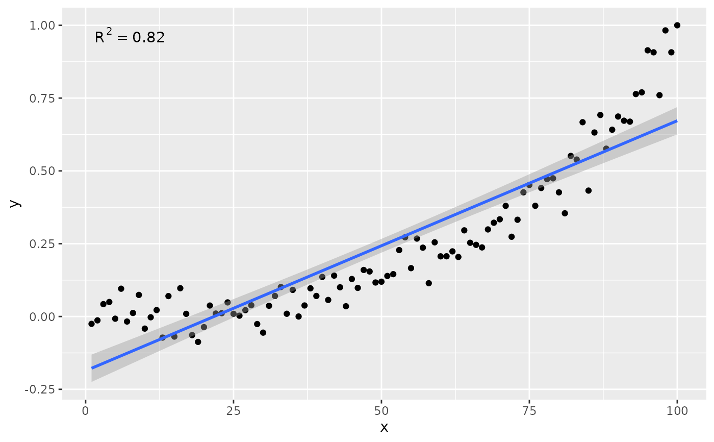
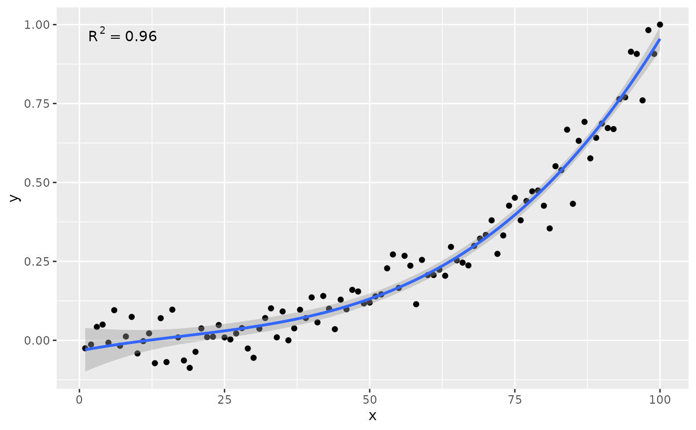
# using defaults
ggplot(my.data, aes(x, y)) +
  geom_point() +
  stat_poly_line() +
  stat_poly_eq()


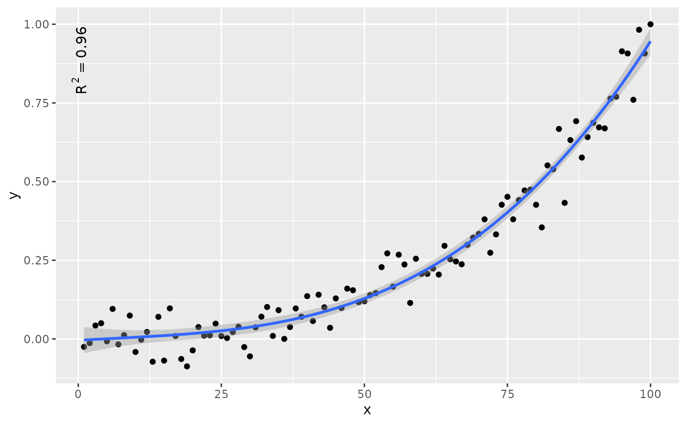
# no weights
ggplot(my.data, aes(x, y)) +
  geom_point() +
  stat_poly_line(formula = formula) +
  stat_poly_eq(formula = formula)


# other labels
ggplot(my.data, aes(x, y)) +
  geom_point() +
  stat_poly_line(formula = formula) +
  stat_poly_eq(use_label("eq"), formula = formula)


# other labels
ggplot(my.data, aes(x, y)) +
  geom_point() +
  stat_poly_line(formula = formula) +
  stat_poly_eq(use_label("eq"), formula = formula, decreasing = TRUE)


ggplot(my.data, aes(x, y)) +
  geom_point() +
  stat_poly_line(formula = formula) +
  stat_poly_eq(use_label("eq", "R2"), formula = formula)


ggplot(my.data, aes(x, y)) +
  geom_point() +
  stat_poly_line(formula = formula) +
  stat_poly_eq(use_label("R2", "R2.CI", "P", "method"), formula = formula)


ggplot(my.data, aes(x, y)) +
  geom_point() +
  stat_poly_line(formula = formula) +
  stat_poly_eq(use_label("R2", "F", "P", "n", sep = "*\"; \"*"),
               formula = formula)


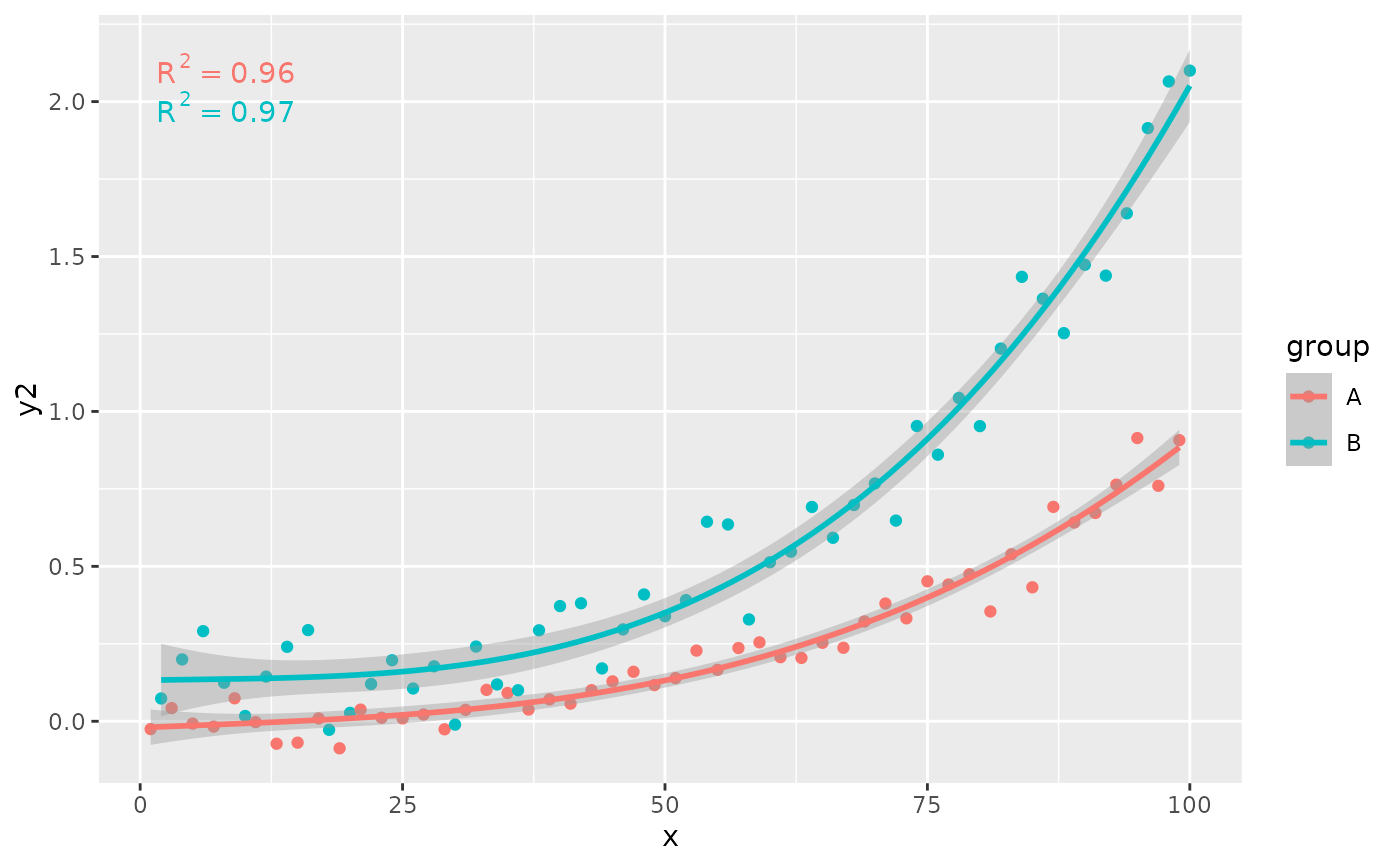
# grouping
ggplot(my.data, aes(x, y2, color = group)) +
  geom_point() +
  stat_poly_line(formula = formula) +
  stat_poly_eq(formula = formula)


# rotation
ggplot(my.data, aes(x, y)) +
  geom_point() +
  stat_poly_line(formula = formula) +
  stat_poly_eq(formula = formula, angle = 90)


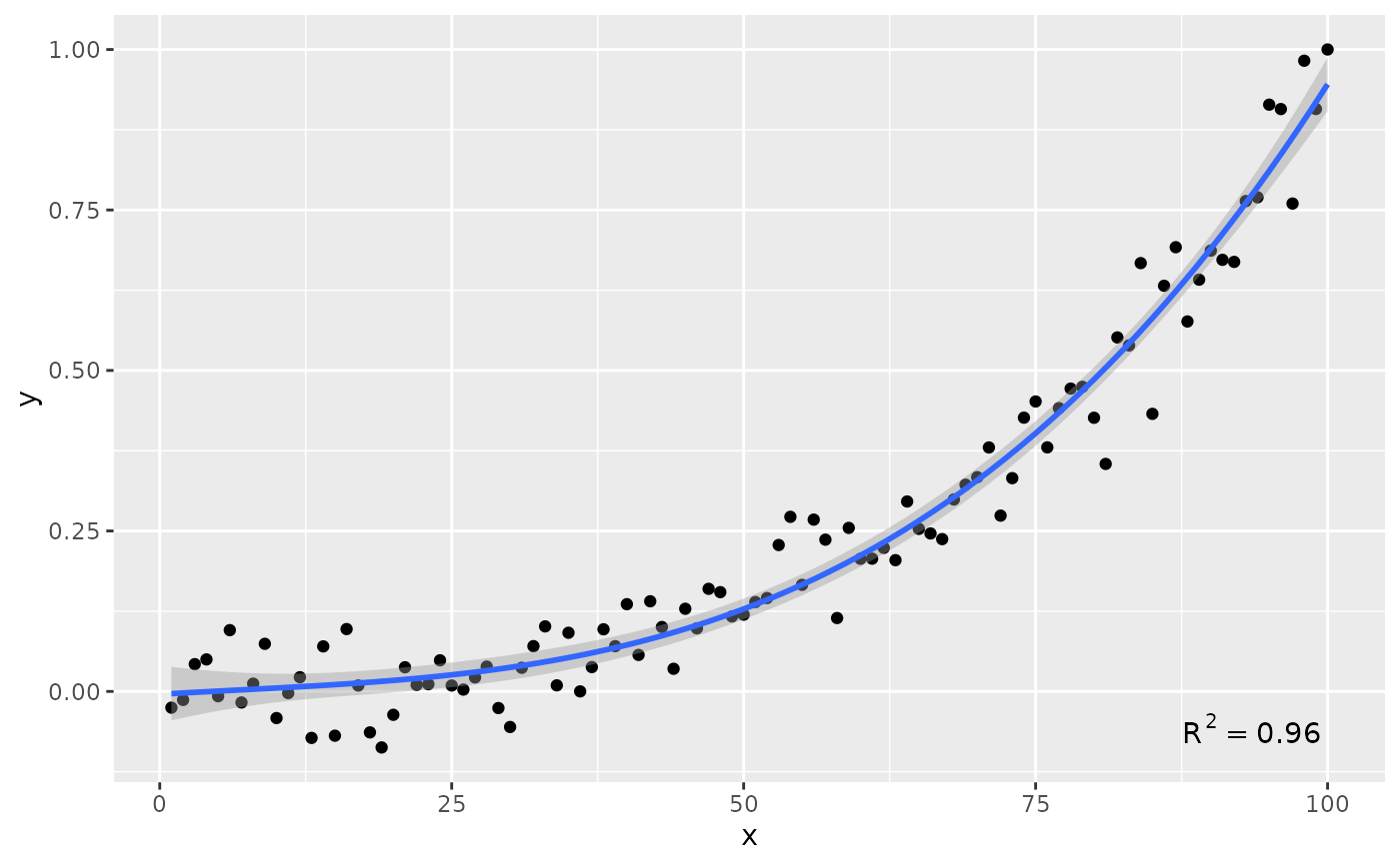
# label location
ggplot(my.data, aes(x, y)) +
  geom_point() +
  stat_poly_line(formula = formula) +
  stat_poly_eq(formula = formula, label.y = "bottom", label.x = "right")


ggplot(my.data, aes(x, y)) +
  geom_point() +
  stat_poly_line(formula = formula) +
  stat_poly_eq(formula = formula, label.y = 0.1, label.x = 0.9)


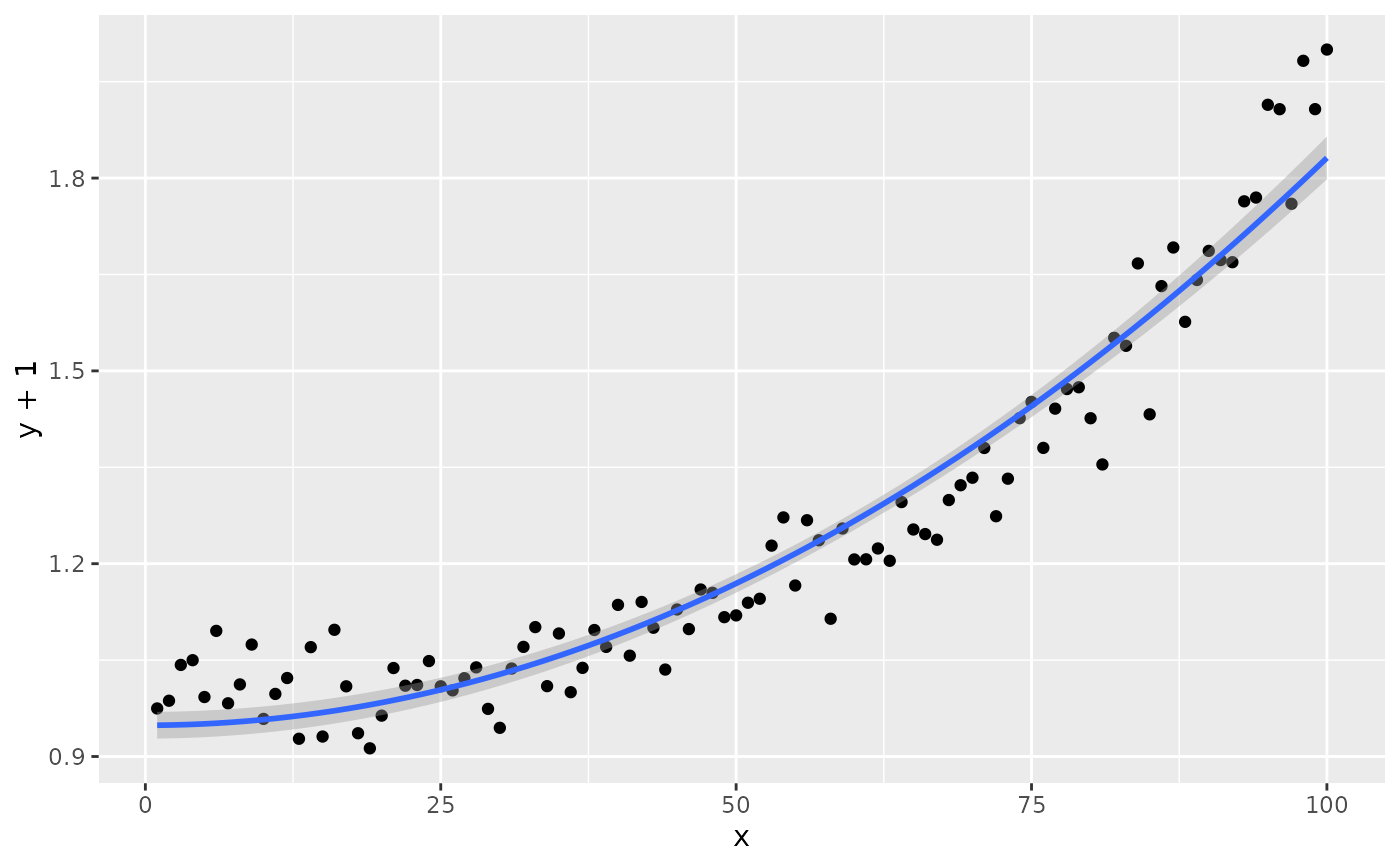
# modifying the explanatory variable within the model formula
# modifying the response variable within aes()
formula.trans <- y ~ I(x^2)
ggplot(my.data, aes(x, y + 1)) +
  geom_point() +
  stat_poly_line(formula = formula.trans) +
  stat_poly_eq(use_label("eq"),
               formula = formula.trans,
               eq.x.rhs = "~x^2",
               eq.with.lhs = "y + 1~~`=`~~")
#> Warning: 'formula' not an increasing polynomial: 'eq.label' is NA!
#> Warning: Removed 1 row containing missing values or values outside the scale range
#> (`geom_text_npc()`).


# using weights
ggplot(my.data, aes(x, y, weight = w)) +
  geom_point() +
  stat_poly_line(formula = formula) +
  stat_poly_eq(formula = formula)


# no weights, 4 digits for R square
ggplot(my.data, aes(x, y)) +
  geom_point() +
  stat_poly_line(formula = formula) +
  stat_poly_eq(formula = formula, rr.digits = 4)


# manually assemble and map a specific label using paste() and aes()
ggplot(my.data, aes(x, y)) +
  geom_point() +
  stat_poly_line(formula = formula) +
  stat_poly_eq(aes(label =  paste(after_stat(rr.label),
                                  after_stat(n.label), sep = "*\", \"*")),
               formula = formula)


# manually assemble and map a specific label using sprintf() and aes()
ggplot(my.data, aes(x, y)) +
  geom_point() +
  stat_poly_line(formula = formula) +
  stat_poly_eq(aes(label =  sprintf("%s*\" with \"*%s*\" and \"*%s",
                                    after_stat(rr.label),
                                    after_stat(f.value.label),
                                    after_stat(p.value.label))),
               formula = formula)


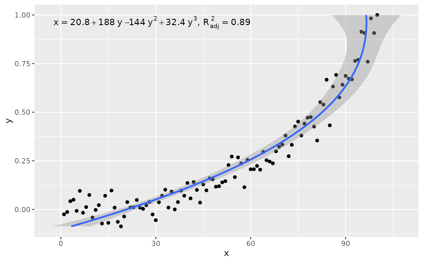
# x on y regression
ggplot(my.data, aes(x, y)) +
  geom_point() +
  stat_poly_line(formula = formula, orientation = "y") +
  stat_poly_eq(use_label("eq", "adj.R2"),
               formula = x ~ poly(y, 3, raw = TRUE))


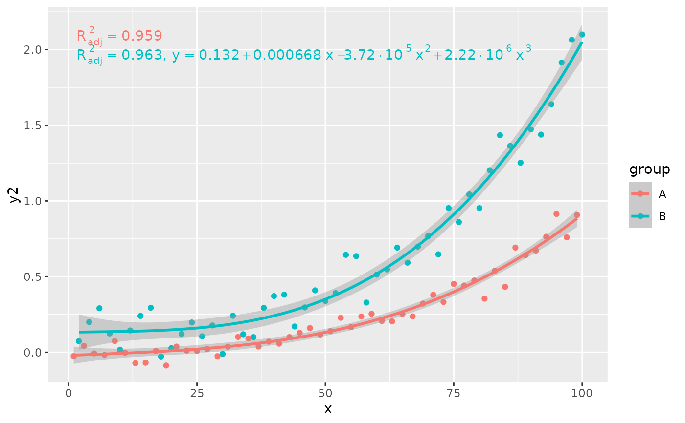
# conditional user specified label
ggplot(my.data, aes(x, y2, color = group)) +
  geom_point() +
  stat_poly_line(formula = formula) +
  stat_poly_eq(aes(label =  ifelse(after_stat(adj.r.squared) > 0.96,
                                   paste(after_stat(adj.rr.label),
                                         after_stat(eq.label),
                                         sep = "*\", \"*"),
                                   after_stat(adj.rr.label))),
               rr.digits = 3,
               formula = formula)


# geom = "text"
ggplot(my.data, aes(x, y)) +
  geom_point() +
  stat_poly_line(formula = formula) +
  stat_poly_eq(geom = "text", label.x = 100, label.y = 0, hjust = 1,
               formula = formula)


# using numeric values
# Here we use columns b_0 ... b_3 for the coefficient estimates
my.format <-
  "b[0]~`=`~%.3g*\", \"*b[1]~`=`~%.3g*\", \"*b[2]~`=`~%.3g*\", \"*b[3]~`=`~%.3g"
ggplot(my.data, aes(x, y)) +
  geom_point() +
  stat_poly_line(formula = formula) +
  stat_poly_eq(formula = formula,
               output.type = "numeric",
               parse = TRUE,
               mapping =
                aes(label = sprintf(my.format,
                                    after_stat(b_0), after_stat(b_1),
                                    after_stat(b_2), after_stat(b_3))))


# Inspecting the returned data using geom_debug()
# This provides a quick way of finding out the names of the variables that
# are available for mapping to aesthetics with after_stat().

gginnards.installed <- requireNamespace("gginnards", quietly = TRUE)

if (gginnards.installed)
  library(gginnards)

if (gginnards.installed)
  ggplot(my.data, aes(x, y)) +
    geom_point() +
    stat_poly_line(formula = formula) +
    stat_poly_eq(formula = formula, geom = "debug")

#> [1] "PANEL 1; group(s) -1; 'draw_function()' input 'data' (head):"
#>   npcx npcy                  label
#> 1   NA   NA italic(R)^2~`=`~"0.96"
#>                                                                                                      eq.label
#> 1 italic(y)~`=`~-0.00450 + 0.00109*~italic(x) - 2.14%*% 10^{-05}*~italic(x)^2 + 1.06%*% 10^{-06}*~italic(x)^3
#>                 rr.label                adj.rr.label      rr.confint.label
#> 1 italic(R)^2~`=`~"0.96" italic(R)[adj]^2~`=`~"0.96" "95% CI [0.95, 0.97]"
#>                 AIC.label               BIC.label
#> 1 plain(AIC)~`=`~"-291.9" plain(BIC)~`=`~"-278.8"
#>                    f.value.label         p.value.label           n.label
#> 1 italic(F)[3*","*96]~`=`~"810." italic(P)~`<`~"0.001" italic(n)~`=`~100
#>   grp.label    method.label r.squared adj.r.squared      p.value   n fm.method
#> 1        -1 "method: lm:qr" 0.9620171     0.9608301 5.110349e-68 100     lm:qr
#>   fm.class                 fm.formula             fm.formula.chr x y PANEL
#> 1       lm y ~ poly(x, 3, raw = TRUE) y ~ poly(x, 3, raw = TRUE) 1 1     1
#>   group orientation
#> 1    -1           x

if (gginnards.installed)
  ggplot(my.data, aes(x, y)) +
    geom_point() +
    stat_poly_line(formula = formula) +
    stat_poly_eq(formula = formula, geom = "debug", output.type = "numeric")

#> [1] "PANEL 1; group(s) -1; 'draw_function()' input 'data' (head):"
#>   npcx npcy label
#> 1   NA   NA      
#>                                                                                                                                                                                                                              coef.ls
#> 1 -4.495631e-03, 1.089644e-03, -2.139937e-05, 1.055387e-06, 2.268244e-02, 1.935252e-03, 4.440449e-05, 2.890821e-07, -1.981987e-01, 5.630500e-01, -4.819189e-01, 3.650820e+00, 8.433087e-01, 5.747135e-01, 6.309604e-01, 4.255076e-04
#>                                                      coefs r.squared
#> 1 -4.495631e-03, 1.089644e-03, -2.139937e-05, 1.055387e-06 0.9620171
#>   rr.confint.level rr.confint.low rr.confint.high adj.r.squared f.value f.df1
#> 1             0.95      0.9464423       0.9696371     0.9608301 810.484     3
#>   f.df2      p.value       AIC      BIC   n rr.label b_0.constant          b_0
#> 1    96 5.110349e-68 -291.8639 -278.838 100                 FALSE -0.004495631
#>           b_1           b_2          b_3 fm.method fm.class
#> 1 0.001089644 -2.139937e-05 1.055387e-06     lm:qr       lm
#>                   fm.formula             fm.formula.chr x y PANEL group
#> 1 y ~ poly(x, 3, raw = TRUE) y ~ poly(x, 3, raw = TRUE) 1 1     1    -1
#>   orientation
#> 1           x

# names of the variables
if (gginnards.installed)
  ggplot(my.data, aes(x, y)) +
    geom_point() +
    stat_poly_line(formula = formula) +
    stat_poly_eq(formula = formula, geom = "debug",
                 summary.fun = colnames)
#> Warning: Ignoring unknown parameters: `summary.fun`

#> [1] "PANEL 1; group(s) -1; 'draw_function()' input 'data' (head):"
#>   npcx npcy                  label
#> 1   NA   NA italic(R)^2~`=`~"0.96"
#>                                                                                                      eq.label
#> 1 italic(y)~`=`~-0.00450 + 0.00109*~italic(x) - 2.14%*% 10^{-05}*~italic(x)^2 + 1.06%*% 10^{-06}*~italic(x)^3
#>                 rr.label                adj.rr.label      rr.confint.label
#> 1 italic(R)^2~`=`~"0.96" italic(R)[adj]^2~`=`~"0.96" "95% CI [0.95, 0.97]"
#>                 AIC.label               BIC.label
#> 1 plain(AIC)~`=`~"-291.9" plain(BIC)~`=`~"-278.8"
#>                    f.value.label         p.value.label           n.label
#> 1 italic(F)[3*","*96]~`=`~"810." italic(P)~`<`~"0.001" italic(n)~`=`~100
#>   grp.label    method.label r.squared adj.r.squared      p.value   n fm.method
#> 1        -1 "method: lm:qr" 0.9620171     0.9608301 5.110349e-68 100     lm:qr
#>   fm.class                 fm.formula             fm.formula.chr x y PANEL
#> 1       lm y ~ poly(x, 3, raw = TRUE) y ~ poly(x, 3, raw = TRUE) 1 1     1
#>   group orientation
#> 1    -1           x

# only data$eq.label
if (gginnards.installed)
  ggplot(my.data, aes(x, y)) +
    geom_point() +
    stat_poly_line(formula = formula) +
    stat_poly_eq(formula = formula, geom = "debug",
                 output.type = "expression",
                 summary.fun = function(x) {x[["eq.label"]]})
#> Warning: Ignoring unknown parameters: `summary.fun`

#> [1] "PANEL 1; group(s) -1; 'draw_function()' input 'data' (head):"
#>   npcx npcy                  label
#> 1   NA   NA italic(R)^2~`=`~"0.96"
#>                                                                                                      eq.label
#> 1 italic(y)~`=`~-0.00450 + 0.00109*~italic(x) - 2.14%*% 10^{-05}*~italic(x)^2 + 1.06%*% 10^{-06}*~italic(x)^3
#>                 rr.label                adj.rr.label      rr.confint.label
#> 1 italic(R)^2~`=`~"0.96" italic(R)[adj]^2~`=`~"0.96" "95% CI [0.95, 0.97]"
#>                 AIC.label               BIC.label
#> 1 plain(AIC)~`=`~"-291.9" plain(BIC)~`=`~"-278.8"
#>                    f.value.label         p.value.label           n.label
#> 1 italic(F)[3*","*96]~`=`~"810." italic(P)~`<`~"0.001" italic(n)~`=`~100
#>   grp.label    method.label r.squared adj.r.squared      p.value   n fm.method
#> 1        -1 "method: lm:qr" 0.9620171     0.9608301 5.110349e-68 100     lm:qr
#>   fm.class                 fm.formula             fm.formula.chr x y PANEL
#> 1       lm y ~ poly(x, 3, raw = TRUE) y ~ poly(x, 3, raw = TRUE) 1 1     1
#>   group orientation
#> 1    -1           x

# only data$eq.label
if (gginnards.installed)
  ggplot(my.data, aes(x, y)) +
    geom_point() +
    stat_poly_line(formula = formula) +
    stat_poly_eq(aes(label = after_stat(eq.label)),
                 formula = formula, geom = "debug",
                 output.type = "markdown",
                 summary.fun = function(x) {x[["eq.label"]]})
#> Warning: Ignoring unknown parameters: `summary.fun`

#> [1] "PANEL 1; group(s) -1; 'draw_function()' input 'data' (head):"
#>   npcx npcy
#> 1   NA   NA
#>                                                                                                                             label
#> 1 _y_ = -0.00450+0.00109&nbsp;_x_-2.14&times;10<sup>-5</sup>&nbsp;_x_<sup>2</sup>+1.06&times;10<sup>-6</sup>&nbsp;_x_<sup>3</sup>
#>                                                                                                                          eq.label
#> 1 _y_ = -0.00450+0.00109&nbsp;_x_-2.14&times;10<sup>-5</sup>&nbsp;_x_<sup>2</sup>+1.06&times;10<sup>-6</sup>&nbsp;_x_<sup>3</sup>
#>                 rr.label                         adj.rr.label
#> 1 _R_<sup>2</sup> = 0.96 _R_<sup>2</sup><sub>adj</sub> = 0.96
#>      rr.confint.label    AIC.label    BIC.label             f.value.label
#> 1 95% CI [0.95, 0.97] AIC = -291.9 BIC = -278.8 _F_<sub>3,96</sub> = 810.
#>   p.value.label   n.label grp.label    method.label r.squared adj.r.squared
#> 1   _P_ < 0.001 _n_ = 100        -1 "method: lm:qr" 0.9620171     0.9608301
#>        p.value   n fm.method fm.class                 fm.formula
#> 1 5.110349e-68 100     lm:qr       lm y ~ poly(x, 3, raw = TRUE)
#>               fm.formula.chr x y PANEL group orientation
#> 1 y ~ poly(x, 3, raw = TRUE) 1 1     1    -1           x

# only data$eq.label
if (gginnards.installed)
  ggplot(my.data, aes(x, y)) +
    geom_point() +
    stat_poly_line(formula = formula) +
    stat_poly_eq(formula = formula, geom = "debug",
                 output.type = "latex",
                 summary.fun = function(x) {x[["eq.label"]]})
#> Warning: Ignoring unknown parameters: `summary.fun`

#> [1] "PANEL 1; group(s) -1; 'draw_function()' input 'data' (head):"
#>   npcx npcy      label
#> 1   NA   NA R^2 = 0.96
#>                                                                             eq.label
#> 1 y = -0.00450 + 0.00109 x - 2.14\\times{} 10^{-05} x^2 + 1.06\\times{} 10^{-06} x^3
#>     rr.label     adj.rr.label    rr.confint.label              AIC.label
#> 1 R^2 = 0.96 R_{adj}^2 = 0.96 95% CI [0.95, 0.97] \\mathrm{AIC} = -291.9
#>                BIC.label   f.value.label p.value.label           n.label
#> 1 \\mathrm{BIC} = -278.8 F_{3,96} = 810.     P < 0.001 \\mathit{n} = 100
#>   grp.label    method.label r.squared adj.r.squared      p.value   n fm.method
#> 1        -1 "method: lm:qr" 0.9620171     0.9608301 5.110349e-68 100     lm:qr
#>   fm.class                 fm.formula             fm.formula.chr x y PANEL
#> 1       lm y ~ poly(x, 3, raw = TRUE) y ~ poly(x, 3, raw = TRUE) 1 1     1
#>   group orientation
#> 1    -1           x

# only data$eq.label
if (gginnards.installed)
  ggplot(my.data, aes(x, y)) +
    geom_point() +
    stat_poly_line(formula = formula) +
    stat_poly_eq(formula = formula, geom = "debug",
                 output.type = "text",
                 summary.fun = function(x) {x[["eq.label"]]})
#> Warning: Ignoring unknown parameters: `summary.fun`

#> [1] "PANEL 1; group(s) -1; 'draw_function()' input 'data' (head):"
#>   npcx npcy      label
#> 1   NA   NA R^2 = 0.96
#>                                                          eq.label   rr.label
#> 1 y = -0.00450 + 0.00109  x - 2.14 10^-05  x^2 + 1.06 10^-06  x^3 R^2 = 0.96
#>       adj.rr.label    rr.confint.label    AIC.label    BIC.label  f.value.label
#> 1 R_{adj}^2 = 0.96 95% CI [0.95, 0.97] AIC = -291.9 BIC = -278.8 F(3,96) = 810.
#>   p.value.label n.label grp.label    method.label r.squared adj.r.squared
#> 1     P < 0.001 n = 100        -1 "method: lm:qr" 0.9620171     0.9608301
#>        p.value   n fm.method fm.class                 fm.formula
#> 1 5.110349e-68 100     lm:qr       lm y ~ poly(x, 3, raw = TRUE)
#>               fm.formula.chr x y PANEL group orientation
#> 1 y ~ poly(x, 3, raw = TRUE) 1 1     1    -1           x

# show the content of a list column
if (gginnards.installed)
  ggplot(my.data, aes(x, y)) +
    geom_point() +
    stat_poly_line(formula = formula) +
    stat_poly_eq(formula = formula, geom = "debug", output.type = "numeric",
                 summary.fun = function(x) {x[["coef.ls"]][[1]]})
#> Warning: Ignoring unknown parameters: `summary.fun`

#> [1] "PANEL 1; group(s) -1; 'draw_function()' input 'data' (head):"
#>   npcx npcy label
#> 1   NA   NA      
#>                                                                                                                                                                                                                              coef.ls
#> 1 -4.495631e-03, 1.089644e-03, -2.139937e-05, 1.055387e-06, 2.268244e-02, 1.935252e-03, 4.440449e-05, 2.890821e-07, -1.981987e-01, 5.630500e-01, -4.819189e-01, 3.650820e+00, 8.433087e-01, 5.747135e-01, 6.309604e-01, 4.255076e-04
#>                                                      coefs r.squared
#> 1 -4.495631e-03, 1.089644e-03, -2.139937e-05, 1.055387e-06 0.9620171
#>   rr.confint.level rr.confint.low rr.confint.high adj.r.squared f.value f.df1
#> 1             0.95      0.9464423       0.9696371     0.9608301 810.484     3
#>   f.df2      p.value       AIC      BIC   n rr.label b_0.constant          b_0
#> 1    96 5.110349e-68 -291.8639 -278.838 100                 FALSE -0.004495631
#>           b_1           b_2          b_3 fm.method fm.class
#> 1 0.001089644 -2.139937e-05 1.055387e-06     lm:qr       lm
#>                   fm.formula             fm.formula.chr x y PANEL group
#> 1 y ~ poly(x, 3, raw = TRUE) y ~ poly(x, 3, raw = TRUE) 1 1     1    -1
#>   orientation
#> 1           x