Predicted line from quantile regression fit

Predicted values are computed and, by default, plotted. Depending on the fit method, a confidence band can be computed and plotted. The confidence band can be interpreted similarly as that produced by stat_smooth() and stat_poly_line().

stat_quant_line(
  mapping = NULL,
  data = NULL,
  geom = "smooth",
  position = "identity",
  ...,
  quantiles = c(0.25, 0.5, 0.75),
  formula = NULL,
  se = length(quantiles) == 1L,
  fm.values = FALSE,
  n = 80,
  method = "rq",
  method.args = list(),
  n.min = 3L,
  level = 0.95,
  type = "direct",
  interval = "confidence",
  na.rm = FALSE,
  orientation = NA,
  show.legend = NA,
  inherit.aes = TRUE
)

Arguments

mapping: The aesthetic mapping, usually constructed with aes. Only needs to be set at the layer level if you are overriding the plot defaults.
data: A layer specific dataset, only needed if you want to override the plot defaults.
geom: The geometric object to use display the data
position: The position adjustment to use for overlapping points on this layer
...: other arguments passed on to layer. This can include aesthetics whose values you want to set, not map. See layer for more details.
quantiles: numeric vector Values in 0..1 indicating the quantiles.
formula: a formula object. Using aesthetic names x and y instead of original variable names.
se: logical Passed to quantreg::predict.rq().
fm.values: logical Add n as a column to returned data? (`FALSE` by default.)
n: Number of points at which to evaluate smoother.
method: function or character If character, "rq", "rqss" or the name of a model fit function are accepted, possibly followed by the fit function's method argument separated by a colon (e.g. "rq:br"). If a function different to rq(), it must accept arguments named formula, data, weights, tau and method and return a model fit object of class rq, rqs or rqss.
method.args: named list with additional arguments passed to rq(), rqss() or to a function passed as argument to method.
n.min: integer Minimum number of distinct values in the explanatory variable (on the rhs of formula) for fitting to the attempted.
level: numeric in range [0..1] Passed to quantreg::predict.rq().
type: character Passed to quantreg::predict.rq().
interval: character Passed to quantreg::predict.rq().
na.rm: a logical indicating whether NA values should be stripped before the computation proceeds.
orientation: character Either "x" or "y" controlling the default for formula.
show.legend: logical. Should this layer be included in the legends? NA, the default, includes if any aesthetics are mapped. FALSE never includes, and TRUE always includes.
inherit.aes: If FALSE, overrides the default aesthetics, rather than combining with them. This is most useful for helper functions that define both data and aesthetics and shouldn't inherit behaviour from the default plot specification, e.g. borders.

Value

The value returned by the statistic is a data frame, that will have n rows of predicted values and and their confidence limits for each quantile, with each quantile in a group. The variables are x and y with y containing predicted values. In addition, quantile and quantile.f indicate the quantile used and and edited group preserves the original grouping adding a new "level" for each quantile. Is se = TRUE, a confidence band is computed and values for it returned in ymax and ymin.

The value returned by the statistic is a data frame, that will have n rows of predicted values and their confidence limits. Optionally it will also include additional values related to the model fit.

Details

stat_quant_line() behaves similarly to ggplot2::stat_smooth() and stat_poly_line() but supports fitting regressions for multiple quantiles in the same plot layer. This statistic interprets the argument passed to formula accepting y as well as x as explanatory variable, matching stat_quant_eq(). While stat_quant_eq() supports only method "rq", stat_quant_line() and stat_quant_band() support both "rq" and "rqss", In the case of "rqss" the model formula makes normally use of qss() to formulate the spline and its constraints.

geom_smooth, which is used by default, treats each axis differently and thus is dependent on orientation. If no argument is passed to formula, it defaults to y ~ x. Formulas with y as explanatory variable are treated as if x was the explanatory variable and orientation = "y".

Package 'ggpmisc' does not define a new geometry matching this statistic as it is enough for the statistic to return suitable x, y, ymin, ymax and group values.

The minimum number of observations with distinct values in the explanatory variable can be set through parameter n.min. The default n.min = 3L is the smallest usable value. However, model fits with very few observations are of little interest and using larger values of n.min than the default is wise.

There are multiple uses for double regression on x and y. For example, when two variables are subject to mutual constrains, it is useful to consider both of them as explanatory and interpret the relationship based on them. So, from version 0.4.1 'ggpmisc' makes it possible to easily implement the approach described by Cardoso (2019) under the name of "Double quantile regression".

Computed variables

`stat_quant_line()` provides the following variables, some of which depend on the orientation:

y *or* x: predicted value
ymin *or* xmin: lower confidence interval around the mean
ymax *or* xmax: upper confidence interval around the mean

If fm.values = TRUE is passed then one column with the number of observations n used for each fit is also included, with the same value in each row within a group. This is wasteful and disabled by default, but provides a simple and robust approach to achieve effects like colouring or hiding of the model fit line based on the number of observations.

Aesthetics

stat_quant_line understands x and y, to be referenced in the formula and weight passed as argument to parameter weights. All three must be mapped to numeric variables. In addition, the aesthetics understood by the geom ("geom_smooth" is the default) are understood and grouping respected.

References

Cardoso, G. C. (2019) Double quantile regression accurately assesses distance to boundary trade-off. Methods in ecology and evolution, 10(8), 1322-1331.

Examples

ggplot(mpg, aes(displ, hwy)) +
  geom_point() +
  stat_quant_line()


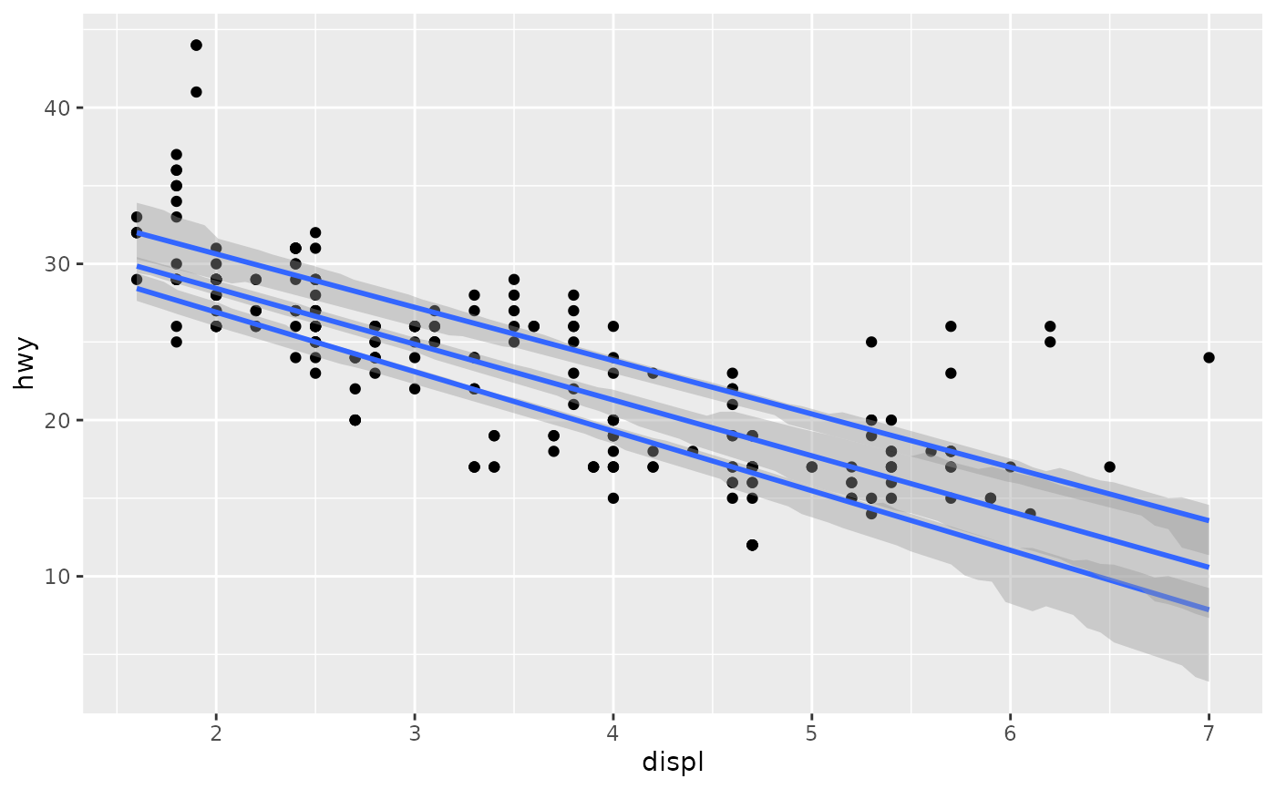
ggplot(mpg, aes(displ, hwy)) +
  geom_point() +
  stat_quant_line(se = TRUE)


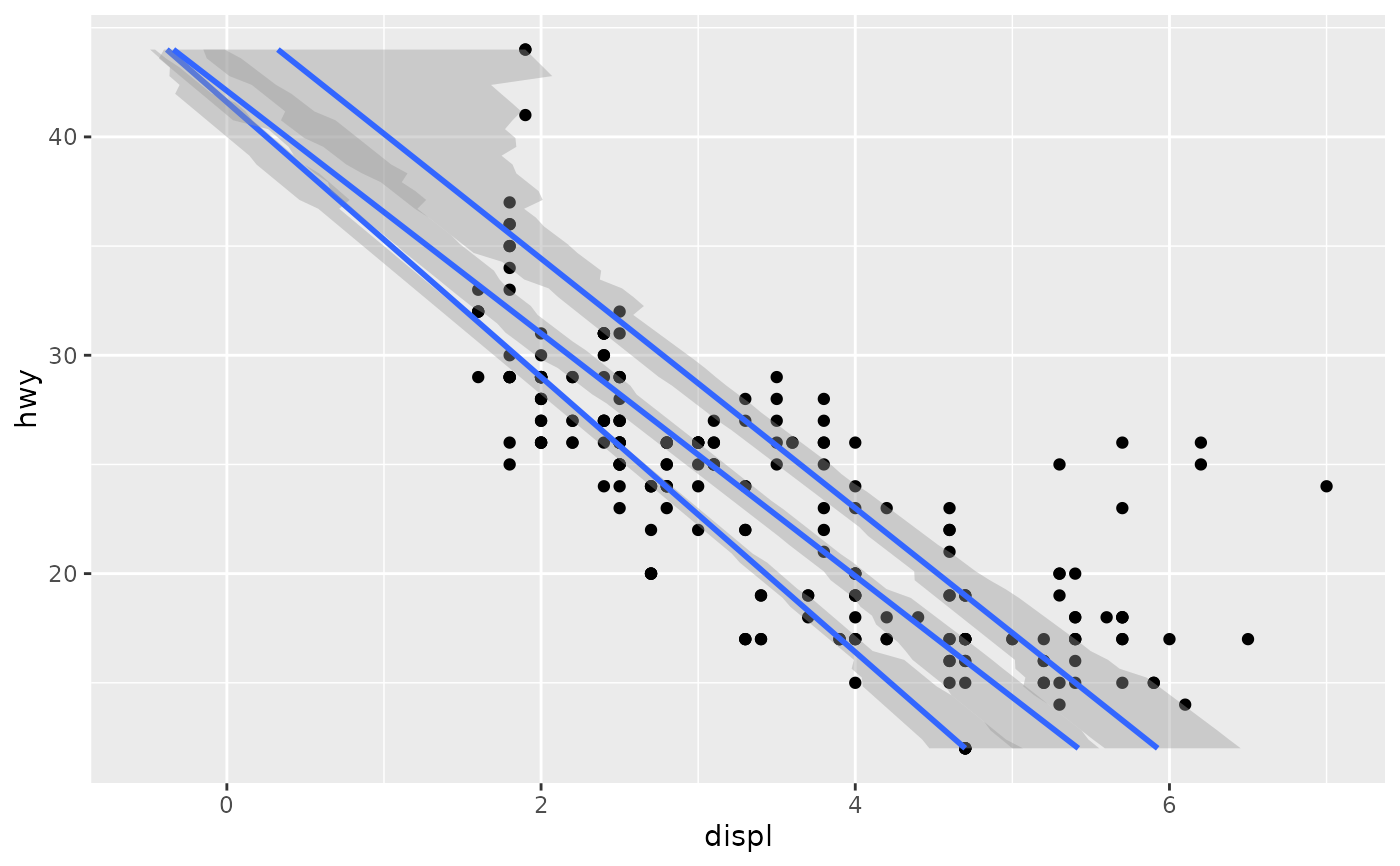
# If you need the fitting to be done along the y-axis set the orientation
ggplot(mpg, aes(displ, hwy)) +
  geom_point() +
  stat_quant_line(orientation = "y")


ggplot(mpg, aes(displ, hwy)) +
  geom_point() +
  stat_quant_line(orientation = "y", se = TRUE)


ggplot(mpg, aes(displ, hwy)) +
  geom_point() +
  stat_quant_line(formula = y ~ x)


ggplot(mpg, aes(displ, hwy)) +
  geom_point() +
  stat_quant_line(formula = x ~ y)


ggplot(mpg, aes(displ, hwy)) +
  geom_point() +
  stat_quant_line(formula = y ~ poly(x, 3))


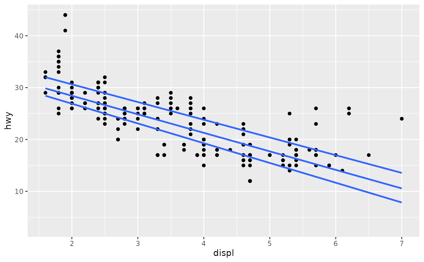
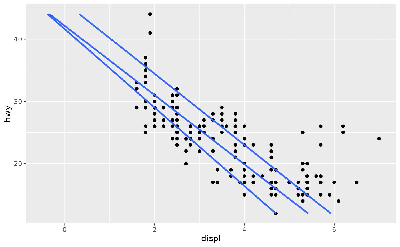
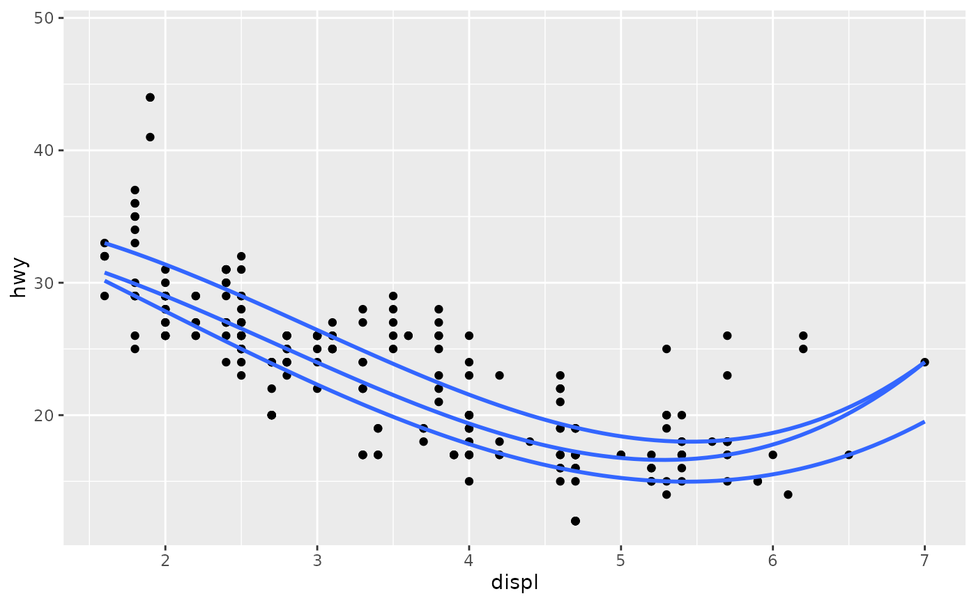
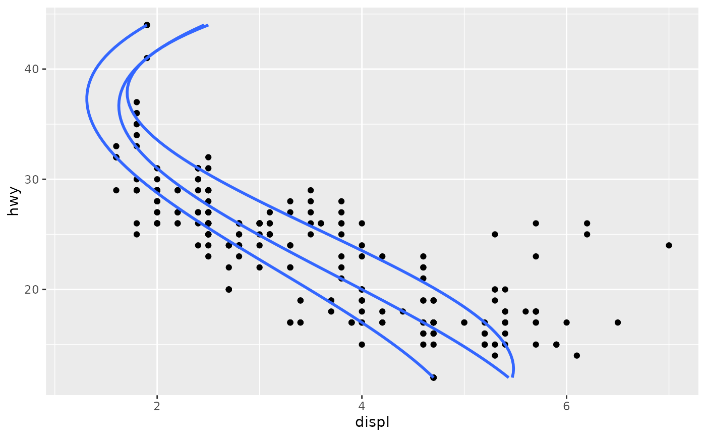
ggplot(mpg, aes(displ, hwy)) +
  geom_point() +
  stat_quant_line(formula = x ~ poly(y, 3))
#> Warning: 9 non-positive fis
#> Warning: 5 non-positive fis


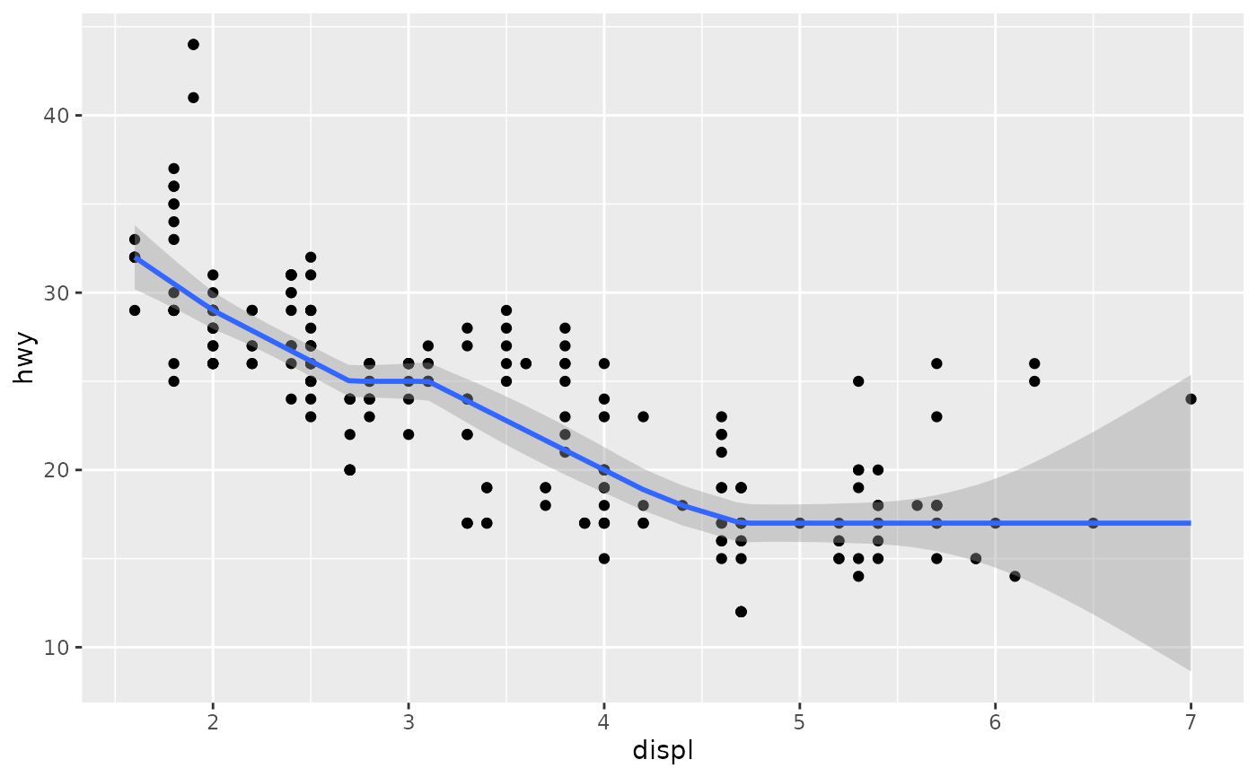
# Instead of rq() we can use rqss() to fit an additive model:
ggplot(mpg, aes(displ, hwy)) +
  geom_point() +
  stat_quant_line(method = "rqss",
                  formula = y ~ qss(x, constraint = "D"),
                  quantiles = 0.5)


ggplot(mpg, aes(displ, hwy)) +
  geom_point() +
  stat_quant_line(method = "rqss",
                  formula = x ~ qss(y, constraint = "D"),
                  quantiles = 0.5)


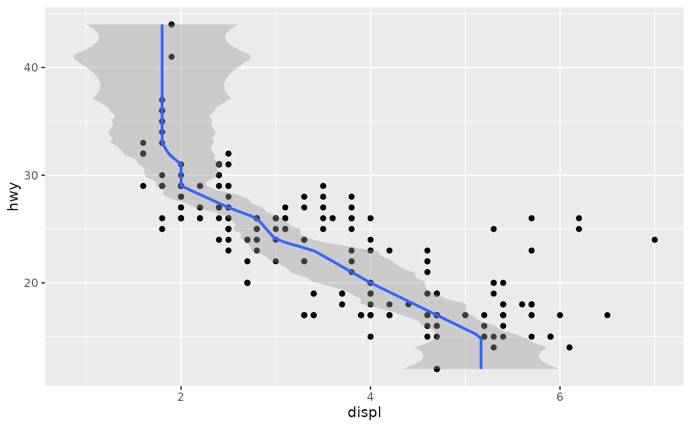
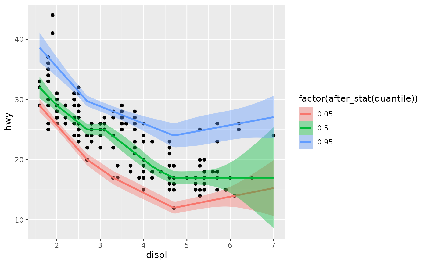
ggplot(mpg, aes(displ, hwy)) +
  geom_point()+
  stat_quant_line(method="rqss",
                  interval="confidence",
                  se = TRUE,
                  mapping = aes(fill = factor(after_stat(quantile)),
                                color = factor(after_stat(quantile))),
                  quantiles=c(0.05,0.5,0.95))
#> Smoothing formula not specified. Using: y ~ qss(x)


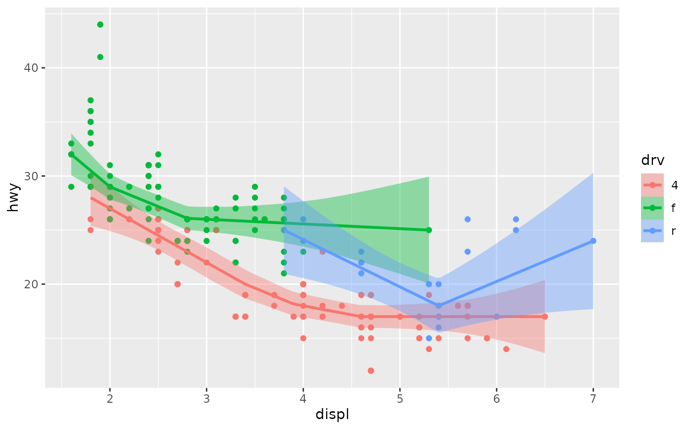
# Smooths are automatically fit to each group (defined by categorical
# aesthetics or the group aesthetic) and for each facet.

ggplot(mpg, aes(displ, hwy, colour = drv, fill = drv)) +
  geom_point() +
  stat_quant_line(method = "rqss",
                  formula = y ~ qss(x, constraint = "V"),
                   quantiles = 0.5)


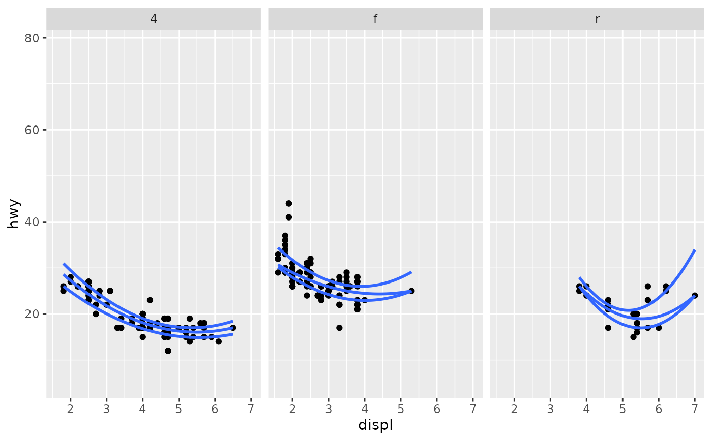
ggplot(mpg, aes(displ, hwy)) +
  geom_point() +
  stat_quant_line(formula = y ~ poly(x, 2)) +
  facet_wrap(~drv)
#> Warning: 1 non-positive fis
#> Warning: 2 non-positive fis


# Inspecting the returned data using geom_debug()
gginnards.installed <- requireNamespace("gginnards", quietly = TRUE)

if (gginnards.installed)
  library(gginnards)

if (gginnards.installed)
  ggplot(mpg, aes(displ, hwy)) +
    stat_quant_line(geom = "debug")

#> [1] "PANEL 1; group(s) -1-0.25, -1-0.5 , -1-0.75; 'draw_function()' input 'data' (head):"
#>     group        x        y quantile     ymin     ymax quantile.f flipped_aes
#> 1 -1-0.25 1.600000 28.42857     0.25 27.62963 29.40000       0.25       FALSE
#> 2 -1-0.25 1.668354 28.16817     0.25 27.35115 29.12658       0.25       FALSE
#> 3 -1-0.25 1.736709 27.90778     0.25 27.07267 28.85316       0.25       FALSE
#> 4 -1-0.25 1.805063 27.64738     0.25 26.77975 28.32801       0.25       FALSE
#> 5 -1-0.25 1.873418 27.38698     0.25 26.50633 28.06054       0.25       FALSE
#> 6 -1-0.25 1.941772 27.12658     0.25 26.23291 27.79307       0.25       FALSE
#>   PANEL orientation
#> 1     1           x
#> 2     1           x
#> 3     1           x
#> 4     1           x
#> 5     1           x
#> 6     1           x

if (gginnards.installed)
  ggplot(mpg, aes(displ, hwy)) +
    stat_quant_line(geom = "debug", fm.values = TRUE)

#> [1] "PANEL 1; group(s) -1-0.25, -1-0.5 , -1-0.75; 'draw_function()' input 'data' (head):"
#>     group        x        y quantile     ymin     ymax   n fm.method fm.formula
#> 1 -1-0.25 1.600000 28.42857     0.25 27.62963 29.40000 234        rq      y ~ x
#> 2 -1-0.25 1.668354 28.16817     0.25 27.35115 29.12658 234        rq      y ~ x
#> 3 -1-0.25 1.736709 27.90778     0.25 27.07267 28.85316 234        rq      y ~ x
#> 4 -1-0.25 1.805063 27.64738     0.25 26.77975 28.32801 234        rq      y ~ x
#> 5 -1-0.25 1.873418 27.38698     0.25 26.50633 28.06054 234        rq      y ~ x
#> 6 -1-0.25 1.941772 27.12658     0.25 26.23291 27.79307 234        rq      y ~ x
#>   fm.formula.chr quantile.f flipped_aes PANEL orientation
#> 1          y ~ x       0.25       FALSE     1           x
#> 2          y ~ x       0.25       FALSE     1           x
#> 3          y ~ x       0.25       FALSE     1           x
#> 4          y ~ x       0.25       FALSE     1           x
#> 5          y ~ x       0.25       FALSE     1           x
#> 6          y ~ x       0.25       FALSE     1           x