Bivariate Cluster Plot (clusplot) Default Method
clusplot.default.RdCreates a bivariate plot visualizing a partition (clustering) of the data. All observation are represented by points in the plot, using principal components or multidimensional scaling. Around each cluster an ellipse is drawn.
Usage
# Default S3 method
clusplot(x, clus, diss = FALSE,
          s.x.2d = mkCheckX(x, diss), stand = FALSE,
          lines = 2, shade = FALSE, color = FALSE,
          labels= 0, plotchar = TRUE,
          col.p = "dark green", col.txt = col.p,
          col.clus = if(color) c(2, 4, 6, 3) else 5, cex = 1, cex.txt = cex,
          span = TRUE,
          add = FALSE,
          xlim = NULL, ylim = NULL,
          main = paste("CLUSPLOT(", deparse1(substitute(x)),")"),
          sub = paste("These two components explain",
             round(100 * var.dec, digits = 2), "% of the point variability."),
          xlab = "Component 1", ylab = "Component 2",
          verbose = getOption("verbose"),
          ...)
Arguments
- x
matrix or data frame, or dissimilarity matrix, depending on the value of the
dissargument.In case of a matrix (alike), each row corresponds to an observation, and each column corresponds to a variable. All variables must be numeric. Missing values (
NAs) are allowed. They are replaced by the median of the corresponding variable. When some variables or some observations contain only missing values, the function stops with a warning message.In case of a dissimilarity matrix,
xis the output ofdaisyordistor a symmetric matrix. Also, a vector of length \(n*(n-1)/2\) is allowed (where \(n\) is the number of observations), and will be interpreted in the same way as the output of the above-mentioned functions. Missing values (NAs) are not allowed.- clus
a vector of length n representing a clustering of
x. For each observation the vector lists the number or name of the cluster to which it has been assigned.clusis often the clustering component of the output ofpam,fannyorclara.- diss
logical indicating if
xwill be considered as a dissimilarity matrix or a matrix of observations by variables (seexarugment above).- s.x.2d
a
listwith components namedx(a \(n \times 2\) matrix; typically something like principal components of original data),labsandvar.dec.
- stand
logical flag: if true, then the representations of the n observations in the 2-dimensional plot are standardized.
- lines
integer out of
0, 1, 2, used to obtain an idea of the distances between ellipses. The distance between two ellipses E1 and E2 is measured along the line connecting the centers \(m1\) and \(m2\) of the two ellipses.In case E1 and E2 overlap on the line through \(m1\) and \(m2\), no line is drawn. Otherwise, the result depends on the value of
lines: If- lines = 0,
no distance lines will appear on the plot;
- lines = 1,
the line segment between \(m1\) and \(m2\) is drawn;
- lines = 2,
a line segment between the boundaries of E1 and E2 is drawn (along the line connecting \(m1\) and \(m2\)).
- shade
logical flag: if TRUE, then the ellipses are shaded in relation to their density. The density is the number of points in the cluster divided by the area of the ellipse.
- color
logical flag: if TRUE, then the ellipses are colored with respect to their density. With increasing density, the colors are light blue, light green, red and purple. To see these colors on the graphics device, an appropriate color scheme should be selected (we recommend a white background).
- labels
integer code, currently one of 0,1,2,3,4 and 5. If
- labels= 0,
no labels are placed in the plot;
- labels= 1,
points and ellipses can be identified in the plot (see
identify);- labels= 2,
all points and ellipses are labelled in the plot;
- labels= 3,
only the points are labelled in the plot;
- labels= 4,
only the ellipses are labelled in the plot.
- labels= 5,
the ellipses are labelled in the plot, and points can be identified.
The levels of the vector
clusare taken as labels for the clusters. The labels of the points are the rownames ofxifxis matrix like. Otherwise (diss = TRUE),xis a vector, point labels can be attached toxas a "Labels" attribute (attr(x,"Labels")), as is done for the output ofdaisy.A possible
namesattribute ofcluswill not be taken into account.- plotchar
logical flag: if TRUE, then the plotting symbols differ for points belonging to different clusters.
- span
logical flag: if TRUE, then each cluster is represented by the ellipse with smallest area containing all its points. (This is a special case of the minimum volume ellipsoid.)
If FALSE, the ellipse is based on the mean and covariance matrix of the same points. While this is faster to compute, it often yields a much larger ellipse.There are also some special cases: When a cluster consists of only one point, a tiny circle is drawn around it. When the points of a cluster fall on a straight line,
span=FALSEdraws a narrow ellipse around it andspan=TRUEgives the exact line segment.- add
logical indicating if ellipses (and labels if
labelsis true) should be added to an already existing plot. If false, neither atitleor sub title, seesub, is written.- col.p
color code(s) used for the observation points.
- col.txt
color code(s) used for the labels (if
labels >= 2).- col.clus
color code for the ellipses (and their labels); only one if color is false (as per default).
- cex, cex.txt
character expansion (size), for the point symbols and point labels, respectively.
- xlim, ylim
numeric vectors of length 2, giving the x- and y- ranges as in
plot.default.- main
main title for the plot; by default, one is constructed.
- sub
sub title for the plot; by default, one is constructed.
- xlab, ylab
x- and y- axis labels for the plot, with defaults.
- verbose
a logical indicating, if there should be extra diagnostic output; mainly for ‘debugging’.
- ...
Further graphical parameters may also be supplied, see
par.
Value
An invisible list with components:
- Distances
When
linesis 1 or 2 we optain a k by k matrix (k is the number of clusters). The element in[i,j]is the distance between ellipse i and ellipse j.
Iflines = 0, then the value of this component isNA.- Shading
A vector of length k (where k is the number of clusters), containing the amount of shading per cluster. Let y be a vector where element i is the ratio between the number of points in cluster i and the area of ellipse i. When the cluster i is a line segment, y[i] and the density of the cluster are set to
NA. Let z be the sum of all the elements of y without the NAs. Then we put shading = y/z *37 + 3 .
Details
clusplot uses function calls
princomp(*, cor = (ncol(x) > 2)) or
cmdscale(*, add=TRUE), respectively, depending on
diss being false or true. These functions are data reduction
techniques to represent the data in a bivariate plot.
Ellipses are then drawn to indicate the clusters. The further layout of the plot is determined by the optional arguments.
Note
When we have 4 or fewer clusters, then the color=TRUE gives
every cluster a different color. When there are more than 4 clusters,
clusplot uses the function pam to cluster the
densities into 4 groups such that ellipses with nearly the same
density get the same color. col.clus specifies the colors used.
The col.p and col.txt arguments, added for R,
are recycled to have length the number of observations.
If col.p has more than one value, using color = TRUE can
be confusing because of a mix of point and ellipse colors.
References
Pison, G., Struyf, A. and Rousseeuw, P.J. (1999)
Displaying a Clustering with CLUSPLOT,
Computational Statistics and Data Analysis, 30, 381–392.
Kaufman, L. and Rousseeuw, P.J. (1990). Finding Groups in Data: An Introduction to Cluster Analysis. Wiley, New York.
Struyf, A., Hubert, M. and Rousseeuw, P.J. (1997). Integrating Robust Clustering Techniques in S-PLUS, Computational Statistics and Data Analysis, 26, 17-37.
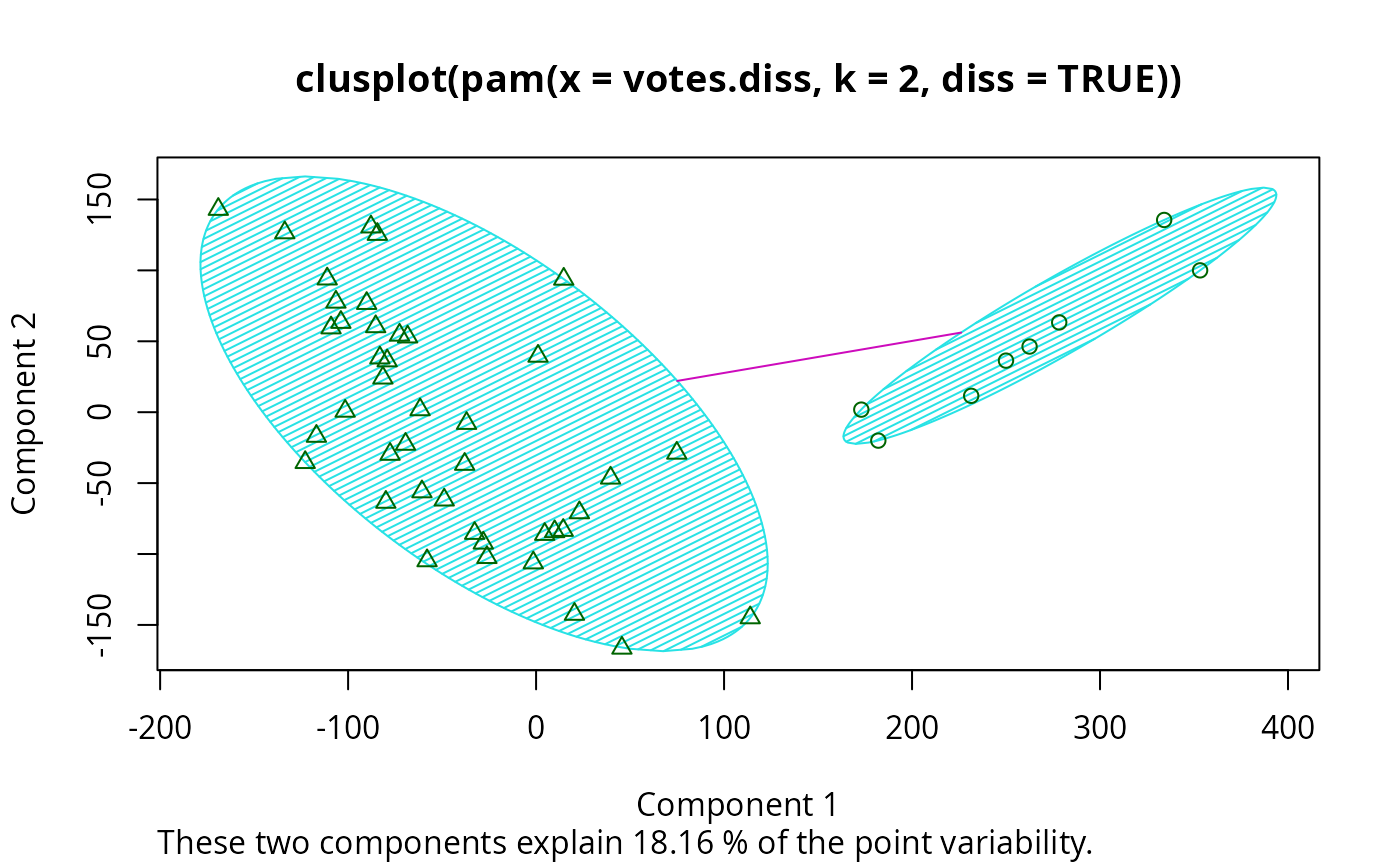
Examples
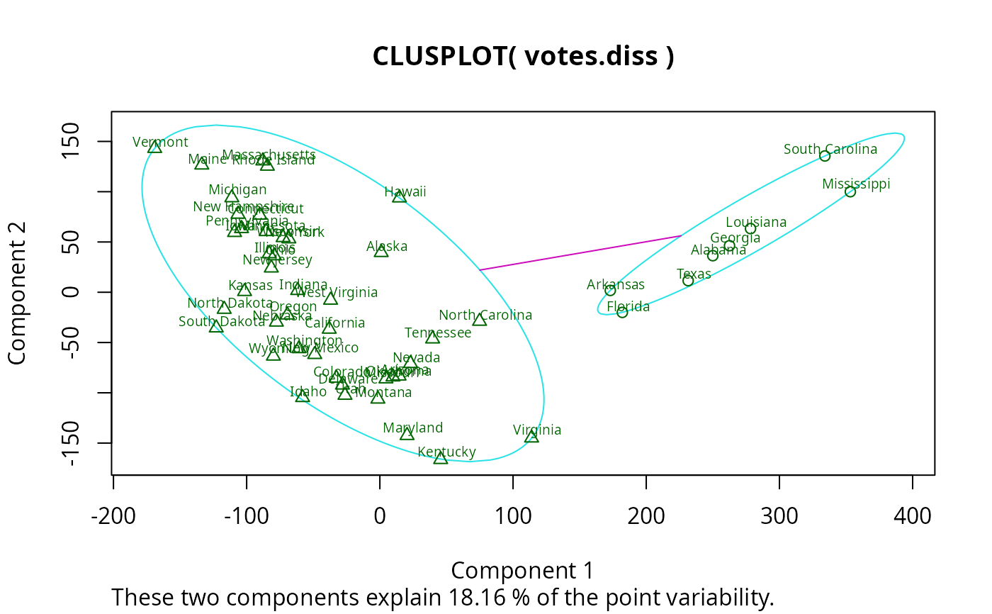
## plotting votes.diss(dissimilarity) in a bivariate plot and
## partitioning into 2 clusters
data(votes.repub)
votes.diss <- daisy(votes.repub)
pamv <- pam(votes.diss, 2, diss = TRUE)
clusplot(pamv, shade = TRUE)
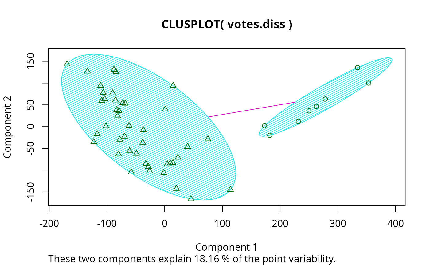
 ## is the same as
votes.clus <- pamv$clustering
clusplot(votes.diss, votes.clus, diss = TRUE, shade = TRUE)
## is the same as
votes.clus <- pamv$clustering
clusplot(votes.diss, votes.clus, diss = TRUE, shade = TRUE)
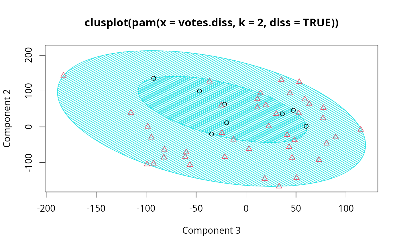
 ## Now look at components 3 and 2 instead of 1 and 2:
str(cMDS <- cmdscale(votes.diss, k=3, add=TRUE))
#> List of 5
#> $ points: num [1:50, 1:3] 249.98 1.03 14.44 173.01 -37.99 ...
#> ..- attr(*, "dimnames")=List of 2
#> .. ..$ : chr [1:50] "Alabama" "Alaska" "Arizona" "Arkansas" ...
#> .. ..$ : NULL
#> $ eig : NULL
#> $ x : NULL
#> $ ac : num 420
#> $ GOF : num [1:2] 0.215 0.215
clusplot(pamv, s.x.2d = list(x=cMDS$points[, c(3,2)],
labs=rownames(votes.repub), var.dec=NA),
shade = TRUE, col.p = votes.clus,
sub="", xlab = "Component 3", ylab = "Component 2")
## Now look at components 3 and 2 instead of 1 and 2:
str(cMDS <- cmdscale(votes.diss, k=3, add=TRUE))
#> List of 5
#> $ points: num [1:50, 1:3] 249.98 1.03 14.44 173.01 -37.99 ...
#> ..- attr(*, "dimnames")=List of 2
#> .. ..$ : chr [1:50] "Alabama" "Alaska" "Arizona" "Arkansas" ...
#> .. ..$ : NULL
#> $ eig : NULL
#> $ x : NULL
#> $ ac : num 420
#> $ GOF : num [1:2] 0.215 0.215
clusplot(pamv, s.x.2d = list(x=cMDS$points[, c(3,2)],
labs=rownames(votes.repub), var.dec=NA),
shade = TRUE, col.p = votes.clus,
sub="", xlab = "Component 3", ylab = "Component 2")
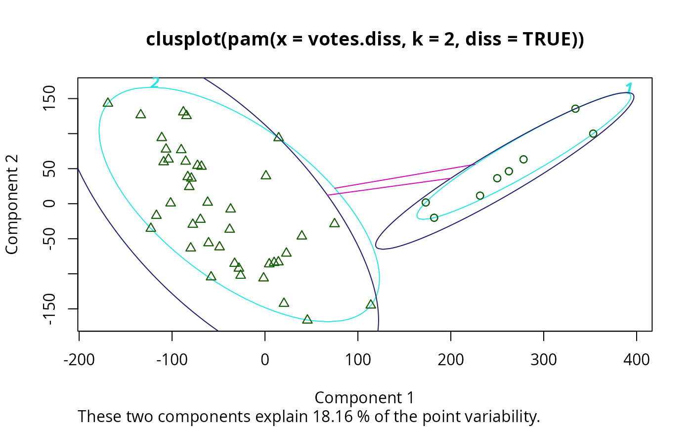
 clusplot(pamv, col.p = votes.clus, labels = 4)# color points and label ellipses
# "simple" cheap ellipses: larger than minimum volume:
# here they are *added* to the previous plot:
clusplot(pamv, span = FALSE, add = TRUE, col.clus = "midnightblue")
clusplot(pamv, col.p = votes.clus, labels = 4)# color points and label ellipses
# "simple" cheap ellipses: larger than minimum volume:
# here they are *added* to the previous plot:
clusplot(pamv, span = FALSE, add = TRUE, col.clus = "midnightblue")
 ## Setting a small *label* size:
clusplot(votes.diss, votes.clus, diss = TRUE, labels = 3, cex.txt = 0.6)
## Setting a small *label* size:
clusplot(votes.diss, votes.clus, diss = TRUE, labels = 3, cex.txt = 0.6)
 if(dev.interactive()) { # uses identify() *interactively* :
clusplot(votes.diss, votes.clus, diss = TRUE, shade = TRUE, labels = 1)
clusplot(votes.diss, votes.clus, diss = TRUE, labels = 5)# ident. only points
}
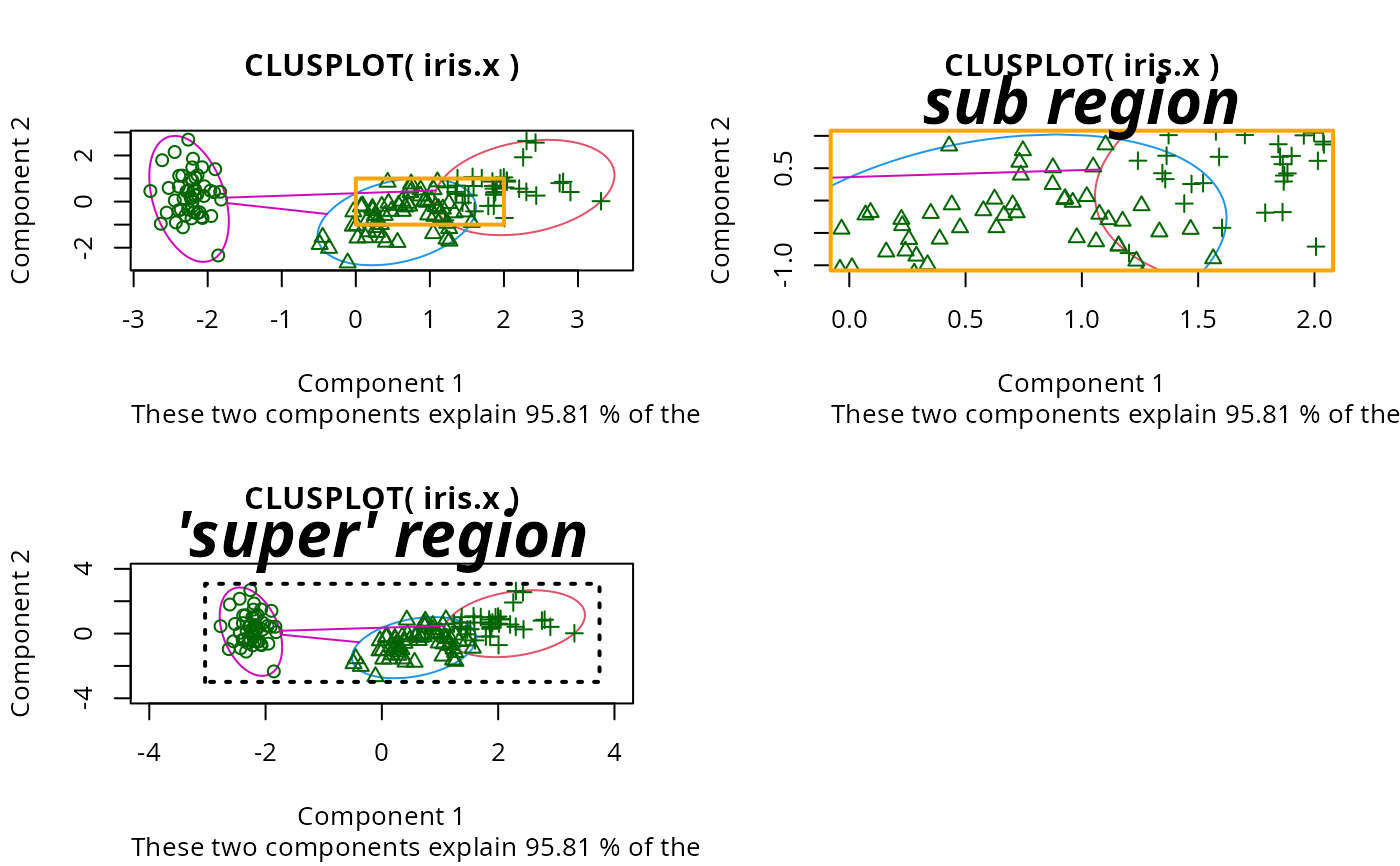
## plotting iris (data frame) in a 2-dimensional plot and partitioning
## into 3 clusters.
data(iris)
iris.x <- iris[, 1:4]
cl3 <- pam(iris.x, 3)$clustering
op <- par(mfrow= c(2,2))
clusplot(iris.x, cl3, color = TRUE)
U <- par("usr")
## zoom in :
rect(0,-1, 2,1, border = "orange", lwd=2)
clusplot(iris.x, cl3, color = TRUE, xlim = c(0,2), ylim = c(-1,1))
box(col="orange",lwd=2); mtext("sub region", font = 4, cex = 2)
## or zoom out :
clusplot(iris.x, cl3, color = TRUE, xlim = c(-4,4), ylim = c(-4,4))
mtext("'super' region", font = 4, cex = 2)
rect(U[1],U[3], U[2],U[4], lwd=2, lty = 3)
# reset graphics
par(op)
if(dev.interactive()) { # uses identify() *interactively* :
clusplot(votes.diss, votes.clus, diss = TRUE, shade = TRUE, labels = 1)
clusplot(votes.diss, votes.clus, diss = TRUE, labels = 5)# ident. only points
}
## plotting iris (data frame) in a 2-dimensional plot and partitioning
## into 3 clusters.
data(iris)
iris.x <- iris[, 1:4]
cl3 <- pam(iris.x, 3)$clustering
op <- par(mfrow= c(2,2))
clusplot(iris.x, cl3, color = TRUE)
U <- par("usr")
## zoom in :
rect(0,-1, 2,1, border = "orange", lwd=2)
clusplot(iris.x, cl3, color = TRUE, xlim = c(0,2), ylim = c(-1,1))
box(col="orange",lwd=2); mtext("sub region", font = 4, cex = 2)
## or zoom out :
clusplot(iris.x, cl3, color = TRUE, xlim = c(-4,4), ylim = c(-4,4))
mtext("'super' region", font = 4, cex = 2)
rect(U[1],U[3], U[2],U[4], lwd=2, lty = 3)
# reset graphics
par(op)