Clustering Large Applications

Computes a "clara" object, a list representing a clustering of the data into k clusters.

Usage

clara(x, k, metric = c("euclidean", "manhattan", "jaccard"),
      stand = FALSE, cluster.only = FALSE, samples = 5,
      sampsize = min(n, 40 + 2 * k), trace = 0, medoids.x = TRUE,
      keep.data = medoids.x, rngR = FALSE, pamLike = FALSE, correct.d = TRUE)

Arguments

x

data matrix or data frame, each row corresponds to an observation, and each column corresponds to a variable. All variables must be numeric (or logical). Missing values (NAs) are allowed.

k

integer, the number of clusters. It is required that $0 < k < n$ where $n$ is the number of observations (i.e., n = nrow(x)).

metric

character string specifying the metric to be used for calculating dissimilarities between observations. The currently available options are "euclidean", "manhattan", "jaccard".

Euclidean distances are root sum-of-squares of differences, and manhattan distances are the sum of absolute differences.

stand

logical, indicating if the measurements in x are standardized before calculating the dissimilarities. Measurements are standardized for each variable (column), by subtracting the variable's mean value and dividing by the variable's mean absolute deviation.

cluster.only

logical; if true, only the clustering will be computed and returned, see details.

samples

integer, say $N$, the number of samples to be drawn from the dataset. The default, N = 5, is rather small for historical (and now back compatibility) reasons and we recommend to set samples an order of magnitude larger.

sampsize

integer, say $j$, the number of observations in each sample. sampsize should be higher than the number of clusters (k) and at most the number of observations ($n =$ nrow(x)). While computational effort is proportional to $j^2$, see note below, it may still be advisable to set $j = $sampsize to a larger value than the (historical) default.

trace

integer indicating a trace level for diagnostic output during the algorithm.

medoids.x

logical indicating if the medoids should be returned, identically to some rows of the input data x. If FALSE, keep.data must be false as well, and the medoid indices, i.e., row numbers of the medoids will still be returned (i.med component), and the algorithm saves space by needing one copy less of x.

keep.data

logical indicating if the (scaled if stand is true) data should be kept in the result. Setting this to FALSE saves memory (and hence time), but disables clusplot()ing of the result. Use medoids.x = FALSE to save even more memory.

rngR

logical indicating if R's random number generator should be used instead of the primitive clara()-builtin one. If true, this also means that each call to clara() returns a different result – though only slightly different in good situations.

pamLike

logical indicating if the “swap” phase (see pam, in C code) should use the same algorithm as pam(). Note that from Kaufman and Rousseeuw's description this should have been true always, but as the original Fortran code and the subsequent port to C has always contained a small one-letter change (a typo according to Martin Maechler) with respect to PAM, the default, pamLike = FALSE has been chosen to remain back compatible rather than “PAM compatible”.

correct.d

logical or integer indicating that—only in the case of NAs present in x—the correct distance computation should be used instead of the wrong formula which has been present in the original Fortran code and been in use up to early 2016.

Because the new correct formula is not back compatible, for the time being, a warning is signalled in this case, unless the user explicitly specifies correct.d.

Value

If cluster.only is false (as by default), an object of class "clara" representing the clustering. See clara.object for details.

If cluster.only is true, the result is the "clustering", an integer vector of length $n$ with entries from 1:k.

Details

clara (for "euclidean" and "manhattan") is fully described in chapter 3 of Kaufman and Rousseeuw (1990). Compared to other partitioning methods such as pam, it can deal with much larger datasets. Internally, this is achieved by considering sub-datasets of fixed size (sampsize) such that the time and storage requirements become linear in $n$ rather than quadratic.

Each sub-dataset is partitioned into k clusters using the same algorithm as in pam.
Once k representative objects have been selected from the sub-dataset, each observation of the entire dataset is assigned to the nearest medoid.

The mean (equivalent to the sum) of the dissimilarities of the observations to their closest medoid is used as a measure of the quality of the clustering. The sub-dataset for which the mean (or sum) is minimal, is retained. A further analysis is carried out on the final partition.

Each sub-dataset is forced to contain the medoids obtained from the best sub-dataset until then. Randomly drawn observations are added to this set until sampsize has been reached.

When cluster.only is true, the result is simply a (possibly named) integer vector specifying the clustering, i.e.,
clara(x,k, cluster.only=TRUE) is the same as
clara(x,k)$clustering but computed more efficiently.

Note

By default, the random sampling is implemented with a very simple scheme (with period $2^{16} = 65536$) inside the Fortran code, independently of R's random number generation, and as a matter of fact, deterministically. Alternatively, we recommend setting rngR = TRUE which uses R's random number generators. Then, clara() results are made reproducible typically by using set.seed() before calling clara.

The storage requirement of clara computation (for small k) is about $O(n \times p) + O(j^2)$ where $j = \code{sampsize}$, and $(n,p) = \code{dim(x)}$. The CPU computing time (again assuming small k) is about $O(n \times p \times j^2 \times N)$, where $N = \code{samples}$.

For “small” datasets, the function pam can be used directly. What can be considered small, is really a function of available computing power, both memory (RAM) and speed. Originally (1990), “small” meant less than 100 observations; in 1997, the authors said “small (say with fewer than 200 observations)”; as of 2006, you can use pam with several thousand observations.

Author

Kaufman and Rousseeuw (see agnes), originally. Metric "jaccard": Kamil Kozlowski (@ownedoutcomes.com) and Kamil Jadeszko. All arguments from trace on, and most R documentation and all tests by Martin Maechler.

Examples

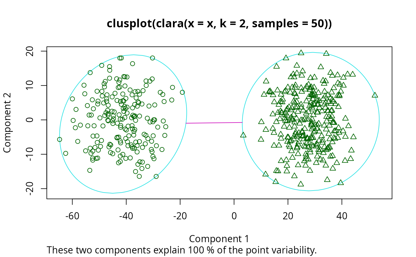
## generate 500 objects, divided into 2 clusters.
x <- rbind(cbind(rnorm(200,0,8), rnorm(200,0,8)),
           cbind(rnorm(300,50,8), rnorm(300,50,8)))
clarax <- clara(x, 2, samples=50)
clarax
#> Call:	 clara(x = x, k = 2, samples = 50) 
#> Medoids:
#>            [,1]       [,2]
#> [1,]  0.8963047  0.5684269
#> [2,] 49.2389207 51.5137030
#> Objective function:	 10.15147
#> Clustering vector: 	 int [1:500] 1 1 1 1 1 1 1 1 1 1 1 1 1 1 1 1 1 1 ...
#> Cluster sizes:	    	 200 300 
#> Best sample:
#>  [1]  10  26  28  34  40  42  46  53  55  63  76  86 115 118 125 140 157 173 175
#> [20] 202 214 262 267 271 272 277 330 347 350 375 382 389 402 413 416 418 434 443
#> [39] 445 449 454 459 470 493
#> 
#> Available components:
#>  [1] "sample"     "medoids"    "i.med"      "clustering" "objective" 
#>  [6] "clusinfo"   "diss"       "call"       "silinfo"    "data"      
clarax$clusinfo
#>      size max_diss  av_diss isolation
#> [1,]  200 24.00382 10.40779 0.3417825
#> [2,]  300 25.62774  9.98059 0.3649051
## using pamLike=TRUE  gives the same (apart from the 'call'):
all.equal(clarax[-8],
          clara(x, 2, samples=50, pamLike = TRUE)[-8])
#> [1] TRUE
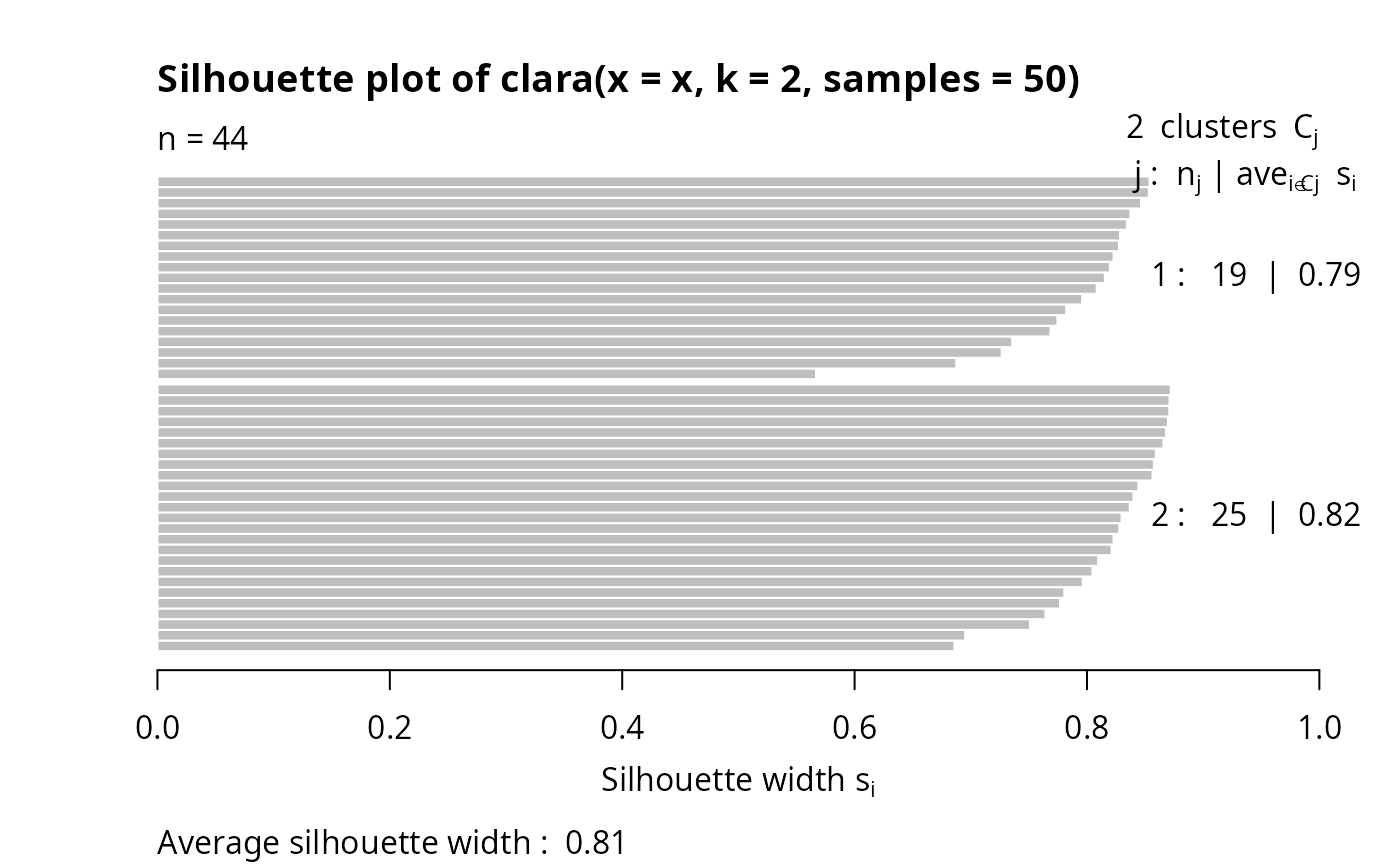
plot(clarax)



## cluster.only = TRUE -- save some memory/time :
clclus <- clara(x, 2, samples=50, cluster.only = TRUE)
stopifnot(identical(clclus, clarax$clustering))


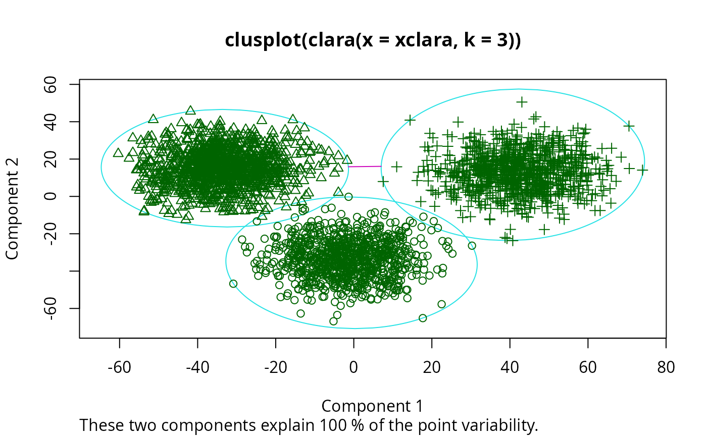
## 'xclara' is an artificial data set with 3 clusters of 1000 bivariate
## objects each.
data(xclara)
(clx3 <- clara(xclara, 3))
#> Call:	 clara(x = xclara, k = 3) 
#> Medoids:
#>             V1        V2
#> [1,]  5.553391 13.306260
#> [2,] 43.198760 60.360720
#> [3,] 74.591890 -6.969018
#> Objective function:	 13.225
#> Clustering vector: 	 int [1:3000] 1 1 1 1 1 1 1 1 1 1 1 1 1 1 1 1 1 1 ...
#> Cluster sizes:	    	 900 1148 952 
#> Best sample:
#>  [1]   20   30   46   91   92  169  179  187  209  223  382  450  555  971 1004
#> [16] 1025 1058 1277 1281 1302 1319 1361 1362 1513 1591 1623 1628 1729 1752 1791
#> [31] 1907 1917 1946 2064 2089 2498 2527 2537 2545 2591 2672 2722 2729 2790 2797
#> [46] 2852
#> 
#> Available components:
#>  [1] "sample"     "medoids"    "i.med"      "clustering" "objective" 
#>  [6] "clusinfo"   "diss"       "call"       "silinfo"    "data"      
## "better" number of samples
cl.3 <- clara(xclara, 3, samples=100)
## but that did not change the result here:
stopifnot(cl.3$clustering == clx3$clustering)
## Plot similar to Figure 5 in Struyf et al (1996)
if (FALSE) plot(clx3, ask = TRUE) # \dontrun{}



## Try 100 times *different* random samples -- for reliability:
nSim <- 100
nCl <- 3 # = no.classes
set.seed(421)# (reproducibility)
cl <- matrix(NA,nrow(xclara), nSim)
for(i in 1:nSim)
   cl[,i] <- clara(xclara, nCl, medoids.x = FALSE, rngR = TRUE)$clustering
tcl <- apply(cl,1, tabulate, nbins = nCl)
## those that are not always in same cluster (5 out of 3000 for this seed):
(iDoubt <- which(apply(tcl,2, function(n) all(n < nSim))))
#>  [1]   30  243  245  309  562  610  708  727  770 1038 1081 1120 1248 1289 1430
#> [16] 1610 1644 1683 1922 2070 2380 2662 2821 2983
if(length(iDoubt)) { # (not for all seeds)
  tabD <- tcl[,iDoubt, drop=FALSE]
  dimnames(tabD) <- list(cluster = paste(1:nCl), obs = format(iDoubt))
  t(tabD) # how many times in which clusters
}
#>       cluster
#> obs     1  2  3
#>     30  4 96  0
#>    243 99  0  1
#>    245 91  0  9
#>    309 99  0  1
#>    562  4  0 96
#>    610 82 18  0
#>    708 87 13  0
#>    727 92  0  8
#>    770  2  1 97
#>   1038 81 19  0
#>   1081 44 56  0
#>   1120 12 88  0
#>   1248 22 78  0
#>   1289  5 95  0
#>   1430  1 99  0
#>   1610 57 43  0
#>   1644 24 76  0
#>   1683  1 99  0
#>   1922 13 87  0
#>   2070  2  0 98
#>   2380  4  0 96
#>   2662  4  0 96
#>   2821  8  0 92
#>   2983  2  0 98