Partitioning Around Medoids
pam.RdPartitioning (clustering) of the data into k clusters “around
medoids”, a more robust version of K-means.
Usage
pam(x, k, diss = inherits(x, "dist"),
    metric = c("euclidean", "manhattan"), <!-- %% FIXME: add "jaccard" -->
    medoids = if(is.numeric(nstart)) "random",
    nstart = if(variant == "faster") 1 else NA,
    stand = FALSE, cluster.only = FALSE,
    do.swap = TRUE,
    keep.diss = !diss && !cluster.only && n < 100,
    keep.data = !diss && !cluster.only,
    variant = c("original", "o_1", "o_2", "f_3", "f_4", "f_5", "faster"),
    pamonce = FALSE, trace.lev = 0)
Arguments
- x
data matrix or data frame, or dissimilarity matrix or object, depending on the value of the
dissargument.In case of a matrix or data frame, each row corresponds to an observation, and each column corresponds to a variable. All variables must be numeric (or logical). Missing values (
NAs) are allowed—as long as every pair of observations has at least one case not missing.In case of a dissimilarity matrix,
xis typically the output ofdaisyordist. Also a vector of length n*(n-1)/2 is allowed (where n is the number of observations), and will be interpreted in the same way as the output of the above-mentioned functions. Missing values (NAs) are not allowed.- k
positive integer specifying the number of clusters, less than the number of observations.
- diss
logical flag: if TRUE (default for
distordissimilarityobjects), thenxwill be considered as a dissimilarity matrix. If FALSE, thenxwill be considered as a matrix of observations by variables.- metric
character string specifying the metric to be used for calculating dissimilarities between observations.
The currently available options are "euclidean" and "manhattan". Euclidean distances are root sum-of-squares of differences, and manhattan distances are the sum of absolute differences. Ifxis already a dissimilarity matrix, then this argument will be ignored.- medoids
NULL (default) or length-
kvector of integer indices (in1:n) specifying initial medoids instead of using the ‘build’ algorithm.- nstart
used only when
medoids = "random": specifies the number of random “starts”; this argument corresponds to the one ofkmeans()(from R's package stats).- stand
logical; if true, the measurements in
xare standardized before calculating the dissimilarities. Measurements are standardized for each variable (column), by subtracting the variable's mean value and dividing by the variable's mean absolute deviation. Ifxis already a dissimilarity matrix, then this argument will be ignored.- cluster.only
logical; if true, only the clustering will be computed and returned, see details.
- do.swap
logical indicating if the swap phase should happen. The default,
TRUE, correspond to the original algorithm. On the other hand, the swap phase is much more computer intensive than the build one for large \(n\), so can be skipped bydo.swap = FALSE.- keep.diss, keep.data
logicals indicating if the dissimilarities and/or input data
xshould be kept in the result. Setting these toFALSEcan give much smaller results and hence even save memory allocation time.- pamonce
logical or integer in
0:6specifying algorithmic short cuts as proposed by Reynolds et al. (2006), and Schubert and Rousseeuw (2019, 2021) see below.- variant
a
characterstring denoting the variant of PAM algorithm to use; a more self-documenting version ofpamoncewhich should be used preferably; note that"faster"not only usespamonce = 6but alsonstart = 1and hencemedoids = "random"by default.- trace.lev
integer specifying a trace level for printing diagnostics during the build and swap phase of the algorithm. Default
0does not print anything; higher values print increasingly more.
Value
an object of class "pam" representing the clustering. See
?pam.object for details.
Details
The basic pam algorithm is fully described in chapter 2 of
Kaufman and Rousseeuw(1990). Compared to the k-means approach in kmeans, the
function pam has the following features: (a) it also accepts a
dissimilarity matrix; (b) it is more robust because it minimizes a sum
of dissimilarities instead of a sum of squared euclidean distances;
(c) it provides a novel graphical display, the silhouette plot (see
plot.partition) (d) it allows to select the number of clusters
using mean(silhouette(pr)[, "sil_width"]) on the result
pr <- pam(..), or directly its component
pr$silinfo$avg.width, see also pam.object.
When cluster.only is true, the result is simply a (possibly
named) integer vector specifying the clustering, i.e.,pam(x,k, cluster.only=TRUE) is the same as pam(x,k)$clustering but computed more efficiently.
The pam-algorithm is based on the search for k
representative objects or medoids among the observations of the
dataset. These observations should represent the structure of the
data. After finding a set of k medoids, k clusters are
constructed by assigning each observation to the nearest medoid. The
goal is to find k representative objects which minimize the sum
of the dissimilarities of the observations to their closest
representative object.
By default, when medoids are not specified, the algorithm first
looks for a good initial set of medoids (this is called the
build phase). Then it finds a local minimum for the
objective function, that is, a solution such that there is no single
switch of an observation with a medoid (i.e. a ‘swap’) that will
decrease the objective (this is called the swap phase).
When the medoids are specified (or randomly generated), their order does not
matter; in general, the algorithms have been designed to not depend on
the order of the observations.
The pamonce option, new in cluster 1.14.2 (Jan. 2012), has been
proposed by Matthias Studer, University of Geneva, based on the
findings by Reynolds et al. (2006) and was extended by Erich Schubert,
TU Dortmund, with the FastPAM optimizations.
The default FALSE (or integer 0) corresponds to the
original “swap” algorithm, whereas pamonce = 1 (or
TRUE), corresponds to the first proposal ....
and pamonce = 2 additionally implements the second proposal as
well.
The key ideas of ‘FastPAM’ (Schubert and Rousseeuw, 2019) are implemented except for the linear approximate build as follows:
pamonce = 3:reduces the runtime by a factor of O(k) by exploiting that points cannot be closest to all current medoids at the same time.
pamonce = 4:additionally allows executing multiple swaps per iteration, usually reducing the number of iterations.
pamonce = 5:adds minor optimizations copied from the
pamonce = 2approach, and is expected to be the fastest of the ‘FastPam’ variants included.
‘FasterPAM’ (Schubert and Rousseeuw, 2021) is implemented via
pamonce = 6:execute each swap which improves results immediately, and hence typically multiple swaps per iteration; this swapping algorithm runs in \(O(n^2)\) rather than \(O(n(n-k)k)\) time which is much faster for all but small \(k\).
In addition, ‘FasterPAM’ uses random initialization of the medoids (instead of the ‘build’ phase) to avoid the \(O(n^2 k)\) initialization cost of the build algorithm. In particular for large k, this yields a much faster algorithm, while preserving a similar result quality.
One may decide to use repeated random initialization by setting
nstart > 1.
Note
For large datasets, pam may need too much memory or too much
computation time since both are \(O(n^2)\). Then,
clara() is preferable, see its documentation.
There is hard limit currently, \(n \le 65536\), at
\(2^{16}\) because for larger \(n\), \(n(n-1)/2\) is larger than
the maximal integer (.Machine$integer.max = \(2^{31} - 1\)).
Author
Kaufman and Rousseeuw's orginal Fortran code was translated to C
and augmented in several ways, e.g. to allow cluster.only=TRUE
or do.swap=FALSE, by Martin Maechler.
Matthias Studer, Univ.Geneva provided the pamonce (1 and 2)
implementation.
Erich Schubert, TU Dortmund contributed the pamonce (3 to 6)
implementation.
References
Reynolds, A., Richards, G., de la Iglesia, B. and Rayward-Smith, V. (1992) Clustering rules: A comparison of partitioning and hierarchical clustering algorithms; Journal of Mathematical Modelling and Algorithms 5, 475–504. doi:10.1007/s10852-005-9022-1 .
Erich Schubert and Peter J. Rousseeuw (2019) Faster k-Medoids Clustering: Improving the PAM, CLARA, and CLARANS Algorithms; SISAP 2020, 171–187. doi:10.1007/978-3-030-32047-8_16 .
Erich Schubert and Peter J. Rousseeuw (2021) Fast and Eager k-Medoids Clustering: O(k) Runtime Improvement of the PAM, CLARA, and CLARANS Algorithms; Preprint, to appear in Information Systems (https://arxiv.org/abs/2008.05171).
See also
agnes for background and references;
pam.object, clara, daisy,
partition.object, plot.partition,
dist.
Examples
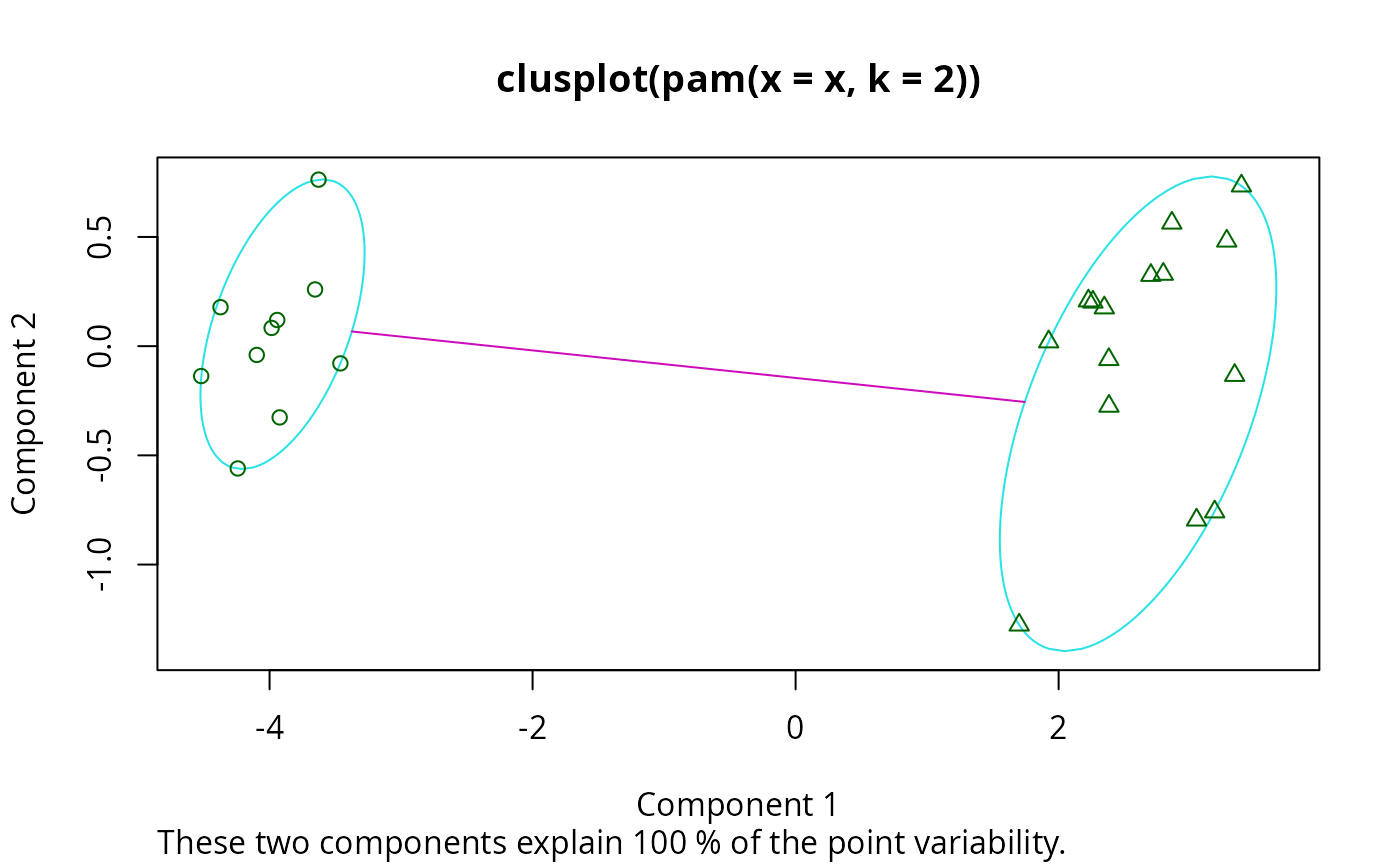
## generate 25 objects, divided into 2 clusters.
set.seed(17) # to get reproducible data:
x <- rbind(cbind(rnorm(10,0,0.5), rnorm(10,0,0.5)),
cbind(rnorm(15,5,0.5), rnorm(15,5,0.5)))
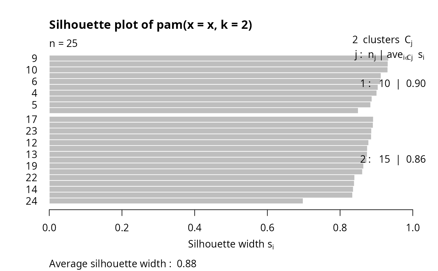
pamx <- pam(x, 2)
pamx # Medoids: '9' and '15' ...
#> Medoids:
#> ID
#> [1,] 9 0.1276185 0.3129772
#> [2,] 15 4.7021222 4.6917243
#> Clustering vector:
#> [1] 1 1 1 1 1 1 1 1 1 1 2 2 2 2 2 2 2 2 2 2 2 2 2 2 2
#> Objective function:
#> build swap
#> 0.7084560 0.5641059
#>
#> Available components:
#> [1] "medoids" "id.med" "clustering" "objective" "isolation"
#> [6] "clusinfo" "silinfo" "diss" "call" "data"
summary(pamx)
#> Medoids:
#> ID
#> [1,] 9 0.1276185 0.3129772
#> [2,] 15 4.7021222 4.6917243
#> Clustering vector:
#> [1] 1 1 1 1 1 1 1 1 1 1 2 2 2 2 2 2 2 2 2 2 2 2 2 2 2
#> Objective function:
#> build swap
#> 0.7084560 0.5641059
#>
#> Numerical information per cluster:
#> size max_diss av_diss diameter separation
#> [1,] 10 0.7669892 0.3999033 1.458134 5.298862
#> [2,] 15 1.5897691 0.6735742 2.626360 5.298862
#>
#> Isolated clusters:
#> L-clusters: character(0)
#> L*-clusters: [1] 1 2
#>
#> Silhouette plot information:
#> cluster neighbor sil_width
#> 9 1 2 0.9333076
#> 2 1 2 0.9318839
#> 10 1 2 0.9313382
#> 3 1 2 0.9127269
#> 6 1 2 0.9120966
#> 7 1 2 0.9044418
#> 4 1 2 0.9011137
#> 1 1 2 0.8877424
#> 5 1 2 0.8842009
#> 8 1 2 0.8501059
#> 17 2 1 0.8916898
#> 18 2 1 0.8910494
#> 23 2 1 0.8866281
#> 15 2 1 0.8861826
#> 12 2 1 0.8787565
#> 21 2 1 0.8752551
#> 13 2 1 0.8749276
#> 11 2 1 0.8734469
#> 19 2 1 0.8648242
#> 16 2 1 0.8617139
#> 22 2 1 0.8402247
#> 20 2 1 0.8392305
#> 14 2 1 0.8365077
#> 25 2 1 0.8344601
#> 24 2 1 0.6983823
#> Average silhouette width per cluster:
#> [1] 0.9048958 0.8555520
#> Average silhouette width of total data set:
#> [1] 0.8752895
#>
#> 300 dissimilarities, summarized :
#> Min. 1st Qu. Median Mean 3rd Qu. Max.
#> 0.03471 0.76270 3.96260 3.76420 6.68460 7.95800
#> Metric : euclidean
#> Number of objects : 25
#>
#> Available components:
#> [1] "medoids" "id.med" "clustering" "objective" "isolation"
#> [6] "clusinfo" "silinfo" "diss" "call" "data"
plot(pamx)
 stopifnot(pamx$id.med == c(9, 15))
stopifnot(identical(pamx$clustering, rep(1:2, c(10, 15))))
## use obs. 1 & 16 as starting medoids -- same result (for seed above, *and* typically) :
(p2m <- pam(x, 2, medoids = c(1,16)))
#> Medoids:
#> ID
#> [1,] 9 0.1276185 0.3129772
#> [2,] 15 4.7021222 4.6917243
#> Clustering vector:
#> [1] 1 1 1 1 1 1 1 1 1 1 2 2 2 2 2 2 2 2 2 2 2 2 2 2 2
#> Objective function:
#> build swap
#> 0.8443840 0.5641059
#>
#> Available components:
#> [1] "medoids" "id.med" "clustering" "objective" "isolation"
#> [6] "clusinfo" "silinfo" "diss" "call" "data"
## no _build_ *and* no _swap_ phase: just cluster all obs. around (1, 16):
p2.s <- pam(x, 2, medoids = c(1,16), do.swap = FALSE)
p2.s
#> Medoids:
#> ID
#> [1,] 1 -0.5075044 0.5903946
#> [2,] 16 5.5799219 5.1271984
#> Clustering vector:
#> [1] 1 1 1 1 1 1 1 1 1 1 2 2 2 2 2 2 2 2 2 2 2 2 2 2 2
#> Objective function:
#> build swap
#> 0.844384 0.844384
#>
#> Available components:
#> [1] "medoids" "id.med" "clustering" "objective" "isolation"
#> [6] "clusinfo" "silinfo" "diss" "call" "data"
keep_nms <- setdiff(names(pamx), c("call", "objective"))# .$objective["build"] differ
stopifnot(p2.s$id.med == c(1,16), # of course
identical(pamx[keep_nms],
p2m[keep_nms]))
p3m <- pam(x, 3, trace.lev = 2)
#> C pam(): computing 301 dissimilarities from 25 x 2 matrix: [Ok]
#> pam()'s bswap(*, s=7.95796, pamonce=0): build 3 medoids:
#> new repr. 25
#> new repr. 9
#> new repr. 18
#> after build: medoids are 9 18 25
#> swp new 23 <-> 25 old; decreasing diss. 12.0983 by -0.855535
#> end{bswap()}, end{cstat()}
## rather stupid initial medoids:
(p3m. <- pam(x, 3, medoids = 3:1, trace.lev = 1))
#> C pam(): computing 301 dissimilarities from 25 x 2 matrix: [Ok]
#> pam()'s bswap(*, s=7.95796, pamonce=0): medoids given; after build: medoids are 1 2 3
#> end{bswap()}, end{cstat()}
#> Medoids:
#> ID
#> [1,] 9 0.1276185 0.3129772
#> [2,] 15 4.7021222 4.6917243
#> [3,] 19 5.1911811 5.6076685
#> Clustering vector:
#> [1] 1 1 1 1 1 1 1 1 1 1 2 2 2 3 2 3 2 2 3 3 2 3 2 2 2
#> Objective function:
#> build swap
#> 4.0910137 0.4520379
#>
#> Available components:
#> [1] "medoids" "id.med" "clustering" "objective" "isolation"
#> [6] "clusinfo" "silinfo" "diss" "call" "data"
pam(daisy(x, metric = "manhattan"), 2, diss = TRUE)
#> Medoids:
#> ID
#> [1,] 2 2
#> [2,] 23 23
#> Clustering vector:
#> [1] 1 1 1 1 1 1 1 1 1 1 2 2 2 2 2 2 2 2 2 2 2 2 2 2 2
#> Objective function:
#> build swap
#> 0.9135804 0.6873926
#>
#> Available components:
#> [1] "medoids" "id.med" "clustering" "objective" "isolation"
#> [6] "clusinfo" "silinfo" "diss" "call"
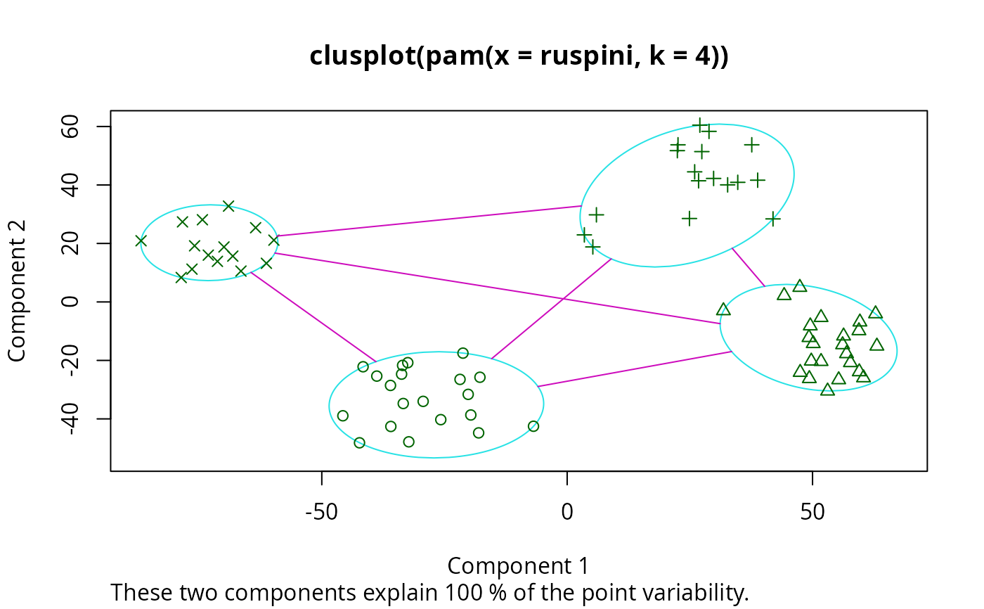
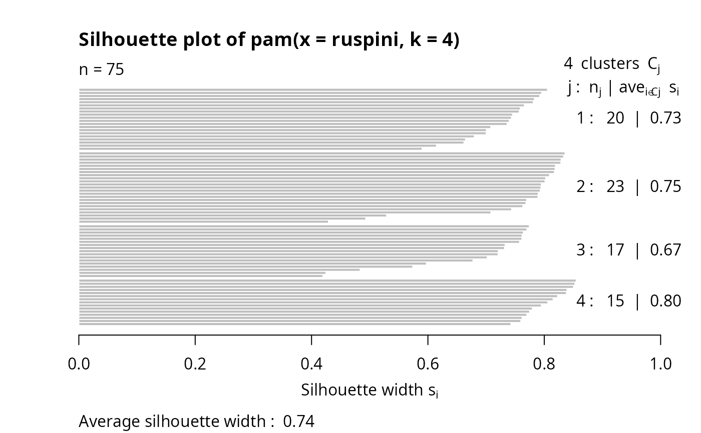
data(ruspini)
## Plot similar to Figure 4 in Stryuf et al (1996)
if (FALSE) plot(pam(ruspini, 4), ask = TRUE) # \dontrun{}
stopifnot(pamx$id.med == c(9, 15))
stopifnot(identical(pamx$clustering, rep(1:2, c(10, 15))))
## use obs. 1 & 16 as starting medoids -- same result (for seed above, *and* typically) :
(p2m <- pam(x, 2, medoids = c(1,16)))
#> Medoids:
#> ID
#> [1,] 9 0.1276185 0.3129772
#> [2,] 15 4.7021222 4.6917243
#> Clustering vector:
#> [1] 1 1 1 1 1 1 1 1 1 1 2 2 2 2 2 2 2 2 2 2 2 2 2 2 2
#> Objective function:
#> build swap
#> 0.8443840 0.5641059
#>
#> Available components:
#> [1] "medoids" "id.med" "clustering" "objective" "isolation"
#> [6] "clusinfo" "silinfo" "diss" "call" "data"
## no _build_ *and* no _swap_ phase: just cluster all obs. around (1, 16):
p2.s <- pam(x, 2, medoids = c(1,16), do.swap = FALSE)
p2.s
#> Medoids:
#> ID
#> [1,] 1 -0.5075044 0.5903946
#> [2,] 16 5.5799219 5.1271984
#> Clustering vector:
#> [1] 1 1 1 1 1 1 1 1 1 1 2 2 2 2 2 2 2 2 2 2 2 2 2 2 2
#> Objective function:
#> build swap
#> 0.844384 0.844384
#>
#> Available components:
#> [1] "medoids" "id.med" "clustering" "objective" "isolation"
#> [6] "clusinfo" "silinfo" "diss" "call" "data"
keep_nms <- setdiff(names(pamx), c("call", "objective"))# .$objective["build"] differ
stopifnot(p2.s$id.med == c(1,16), # of course
identical(pamx[keep_nms],
p2m[keep_nms]))
p3m <- pam(x, 3, trace.lev = 2)
#> C pam(): computing 301 dissimilarities from 25 x 2 matrix: [Ok]
#> pam()'s bswap(*, s=7.95796, pamonce=0): build 3 medoids:
#> new repr. 25
#> new repr. 9
#> new repr. 18
#> after build: medoids are 9 18 25
#> swp new 23 <-> 25 old; decreasing diss. 12.0983 by -0.855535
#> end{bswap()}, end{cstat()}
## rather stupid initial medoids:
(p3m. <- pam(x, 3, medoids = 3:1, trace.lev = 1))
#> C pam(): computing 301 dissimilarities from 25 x 2 matrix: [Ok]
#> pam()'s bswap(*, s=7.95796, pamonce=0): medoids given; after build: medoids are 1 2 3
#> end{bswap()}, end{cstat()}
#> Medoids:
#> ID
#> [1,] 9 0.1276185 0.3129772
#> [2,] 15 4.7021222 4.6917243
#> [3,] 19 5.1911811 5.6076685
#> Clustering vector:
#> [1] 1 1 1 1 1 1 1 1 1 1 2 2 2 3 2 3 2 2 3 3 2 3 2 2 2
#> Objective function:
#> build swap
#> 4.0910137 0.4520379
#>
#> Available components:
#> [1] "medoids" "id.med" "clustering" "objective" "isolation"
#> [6] "clusinfo" "silinfo" "diss" "call" "data"
pam(daisy(x, metric = "manhattan"), 2, diss = TRUE)
#> Medoids:
#> ID
#> [1,] 2 2
#> [2,] 23 23
#> Clustering vector:
#> [1] 1 1 1 1 1 1 1 1 1 1 2 2 2 2 2 2 2 2 2 2 2 2 2 2 2
#> Objective function:
#> build swap
#> 0.9135804 0.6873926
#>
#> Available components:
#> [1] "medoids" "id.med" "clustering" "objective" "isolation"
#> [6] "clusinfo" "silinfo" "diss" "call"
data(ruspini)
## Plot similar to Figure 4 in Stryuf et al (1996)
if (FALSE) plot(pam(ruspini, 4), ask = TRUE) # \dontrun{}