Weighted Statistical Estimates

These functions compute various weighted versions of standard estimators. In most cases the weights vector is a vector the same length of x, containing frequency counts that in effect expand x by these counts. weights can also be sampling weights, in which setting normwt to TRUE will often be appropriate. This results in making weights sum to the length of the non-missing elements in x. normwt=TRUE thus reflects the fact that the true sample size is the length of the x vector and not the sum of the original values of weights (which would be appropriate had normwt=FALSE). When weights is all ones, the estimates are all identical to unweighted estimates (unless one of the non-default quantile estimation options is specified to wtd.quantile). When missing data have already been deleted for, x, weights, and (in the case of wtd.loess.noiter) y, specifying na.rm=FALSE will save computation time. Omitting the weights argument or specifying NULL or a zero-length vector will result in the usual unweighted estimates.

wtd.mean, wtd.var, and wtd.quantile compute weighted means, variances, and quantiles, respectively. wtd.Ecdf computes a weighted empirical distribution function. wtd.table computes a weighted frequency table (although only one stratification variable is supported at present). wtd.rank computes weighted ranks, using mid–ranks for ties. This can be used to obtain Wilcoxon tests and rank correlation coefficients. wtd.loess.noiter is a weighted version of loess.smooth when no iterations for outlier rejection are desired. This results in especially good smoothing when y is binary. wtd.quantile removes any observations with zero weight at the beginning. Previously, these were changing the quantile estimates.

num.denom.setup is a utility function that allows one to deal with observations containing numbers of events and numbers of trials, by outputting two observations when the number of events and non-events (trials - events) exceed zero. A vector of subscripts is generated that will do the proper duplications of observations, and a new binary variable y is created along with usual cell frequencies (weights) for each of the y=0, y=1 cells per observation.

Usage

wtd.mean(x, weights=NULL, normwt="ignored", na.rm=TRUE)
wtd.var(x, weights=NULL, normwt=FALSE, na.rm=TRUE,
        method=c('unbiased', 'ML'))
wtd.quantile(x, weights=NULL, probs=c(0, .25, .5, .75, 1), 
             type=c('quantile','(i-1)/(n-1)','i/(n+1)','i/n'), 
             normwt=FALSE, na.rm=TRUE)
wtd.Ecdf(x, weights=NULL, 
         type=c('i/n','(i-1)/(n-1)','i/(n+1)'), 
         normwt=FALSE, na.rm=TRUE)
wtd.table(x, weights=NULL, type=c('list','table'), 
          normwt=FALSE, na.rm=TRUE)
wtd.rank(x, weights=NULL, normwt=FALSE, na.rm=TRUE)
wtd.loess.noiter(x, y, weights=rep(1,n),
                 span=2/3, degree=1, cell=.13333, 
                 type=c('all','ordered all','evaluate'), 
                 evaluation=100, na.rm=TRUE)
num.denom.setup(num, denom)

Arguments

x: a numeric vector (may be a character or category or factor vector for wtd.table)
num: vector of numerator frequencies
denom: vector of denominators (numbers of trials)
weights: a numeric vector of weights
normwt: specify normwt=TRUE to make weights sum to length(x) after deletion of NAs. If weights are frequency weights, then normwt should be FALSE, and if weights are normalization (aka reliability) weights, then normwt should be TRUE. In the case of the former, no check is made that weights are valid frequencies.
na.rm: set to FALSE to suppress checking for NAs
method: determines the estimator type; if 'unbiased' (the default) then the usual unbiased estimate (using Bessel's correction) is returned, if 'ML' then it is the maximum likelihood estimate for a Gaussian distribution. In the case of the latter, the normwt argument has no effect. Uses stats:cov.wt for both methods.
probs: a vector of quantiles to compute. Default is 0 (min), .25, .5, .75, 1 (max).
type: For wtd.quantile, type defaults to quantile to use the same interpolated order statistic method as quantile. Set type to "(i-1)/(n-1)","i/(n+1)", or "i/n" to use the inverse of the empirical distribution function, using, respectively, (wt - 1)/T, wt/(T+1), or wt/T, where wt is the cumulative weight and T is the total weight (usually total sample size). These three values of type are the possibilities for wtd.Ecdf. For wtd.table the default type is "list", meaning that the function is to return a list containing two vectors: x is the sorted unique values of x and sum.of.weights is the sum of weights for that x. This is the default so that you don't have to convert the names attribute of the result that can be obtained with type="table" to a numeric variable when x was originally numeric. type="table" for wtd.table results in an object that is the same structure as those returned from table. For wtd.loess.noiter the default type is "all", indicating that the function is to return a list containing all the original values of x (including duplicates and without sorting) and the smoothed y values corresponding to them. Set type="ordered all" to sort by x, and type="evaluate" to evaluate the smooth only at evaluation equally spaced points between the observed limits of x.
y: a numeric vector the same length as x
span, degree, cell, evaluation: see loess.smooth. The default is linear (degree=1) and 100 points to evaluation (if type="evaluate").

Value

wtd.mean and wtd.var return scalars. wtd.quantile returns a vector the same length as probs. wtd.Ecdf returns a list whose elements x and Ecdf correspond to unique sorted values of x. If the first CDF estimate is greater than zero, a point (min(x),0) is placed at the beginning of the estimates. See above for wtd.table. wtd.rank returns a vector the same length as x (after removal of NAs, depending on na.rm). See above for wtd.loess.noiter.

Details

The functions correctly combine weights of observations having duplicate values of x before computing estimates.

When normwt=FALSE the weighted variance will not equal the unweighted variance even if the weights are identical. That is because of the subtraction of 1 from the sum of the weights in the denominator of the variance formula. If you want the weighted variance to equal the unweighted variance when weights do not vary, use normwt=TRUE. The articles by Gatz and Smith discuss alternative approaches, to arrive at estimators of the standard error of a weighted mean.

wtd.rank does not handle NAs as elegantly as rank if weights is specified.

Author

Frank Harrell
Department of Biostatistics
Vanderbilt University School of Medicine
fh@fharrell.com
Benjamin Tyner
btyner@gmail.com

References

Research Triangle Institute (1995): SUDAAN User's Manual, Release 6.40, pp. 8-16 to 8-17.

Gatz DF, Smith L (1995): The standard error of a weighted mean concentration–I. Bootstrapping vs other methods. Atmospheric Env 11:1185-1193.

Gatz DF, Smith L (1995): The standard error of a weighted mean concentration–II. Estimating confidence intervals. Atmospheric Env 29:1195-1200.

https://en.wikipedia.org/wiki/Weighted_arithmetic_mean

Examples

set.seed(1)
x <- runif(500)
wts <- sample(1:6, 500, TRUE)
std.dev <- sqrt(wtd.var(x, wts))
wtd.quantile(x, wts)
#>      0%     25%     50%     75%    100% 
#> 0.00184 0.26024 0.46155 0.73964 0.99608 
death <- sample(0:1, 500, TRUE)
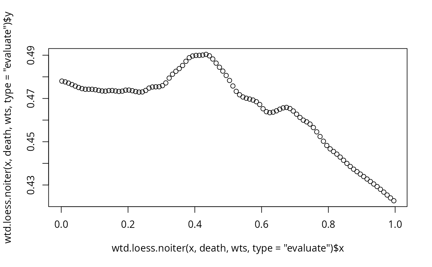
plot(wtd.loess.noiter(x, death, wts, type='evaluate'))

describe(~x, weights=wts)
#> x 
#> 
#>  2  Variables      500  Observations
#> --------------------------------------------------------------------------------
#> x 
#>        n  missing distinct     Info     Mean      .05      .10      .25 
#>     1780        0      500        1   0.4949  0.07068  0.12169  0.26024 
#>      .50      .75      .90      .95 
#>  0.46155  0.73964  0.91037  0.95373 
#> 
#> lowest : 0.00183686 0.00193283 0.0111495  0.0130776  0.0133903 
#> highest: 0.991839   0.991906   0.992684   0.993749   0.996077  
#> --------------------------------------------------------------------------------
#> (weights) 
#>        n  missing distinct     Info     Mean 
#>     1780        0        6    0.949    4.385 
#>                                               
#> Value          1     2     3     4     5     6
#> Frequency     79   174   219   328   470   510
#> Proportion 0.044 0.098 0.123 0.184 0.264 0.287
#> --------------------------------------------------------------------------------
# describe uses wtd.mean, wtd.quantile, wtd.table
xg <- cut2(x,g=4)
table(xg)
#> xg
#> [0.00184,0.258) [0.25817,0.476) [0.47635,0.740) [0.73964,0.996] 
#>             125             125             125             125 
wtd.table(xg, wts, type='table')
#> [0.00184,0.258) [0.25817,0.476) [0.47635,0.740) [0.73964,0.996] 
#>             444             467             421             448 

# Here is a method for getting stratified weighted means
y <- runif(500)
g <- function(y) wtd.mean(y[,1],y[,2])
summarize(cbind(y, wts), llist(xg), g, stat.name='y')
#>                xg     y
#> 1 [0.00184,0.258) 0.444
#> 2 [0.25817,0.476) 0.500
#> 3 [0.47635,0.740) 0.512
#> 4 [0.73964,0.996] 0.496

# Empirically determine how methods used by wtd.quantile match with
# methods used by quantile, when all weights are unity
set.seed(1)
u <-  eval(formals(wtd.quantile)$type)
v <- as.character(1:9)
r <- matrix(0, nrow=length(u), ncol=9, dimnames=list(u,v))

for(n in c(8, 13, 22, 29))
  {
    x <- rnorm(n)
    for(i in 1:5) {
      probs <- sort( runif(9))
      for(wtype in u) {
        wq <- wtd.quantile(x, type=wtype, weights=rep(1,length(x)), probs=probs)
        for(qtype in 1:9) {
          rq <- quantile(x, type=qtype, probs=probs)
          r[wtype, qtype] <- max(r[wtype,qtype], max(abs(wq-rq)))
        }
      }
    }
  }

r
#>                 1     2     3        4     5        6        7     8     9
#> quantile    0.573 0.573 0.755 5.02e-01 0.373 6.42e-01 0.00e+00 0.472 0.442
#> (i-1)/(n-1) 0.573 0.573 0.755 5.02e-01 0.373 6.42e-01 8.88e-16 0.472 0.442
#> i/(n+1)     0.709 0.709 0.857 7.20e-01 0.321 4.44e-16 6.42e-01 0.214 0.241
#> i/n         0.777 0.777 0.409 4.44e-16 0.428 7.20e-01 5.02e-01 0.546 0.517

# Restructure data to generate a dichotomous response variable
# from records containing numbers of events and numbers of trials
num   <- c(10,NA,20,0,15)   # data are 10/12 NA/999 20/20 0/25 15/35
denom <- c(12,999,20,25,35)
w     <- num.denom.setup(num, denom)
w
#> $subs
#> [1] 1 3 5 1 4 5
#> 
#> $weights
#> [1] 10 20 15  2 25 20
#> 
#> $y
#> [1] 1 1 1 0 0 0
#> 
# attach(my.data.frame[w$subs,])