Graphical Summarization of Continuous Variables Against a Response

summaryRc is a continuous version of summary.formula with method='response'. It uses the plsmo function to compute the possibly stratified lowess nonparametric regression estimates, and plots them along with the data density, with selected quantiles of the overall distribution (over strata) of each x shown as arrows on top of the graph. All the x variables must be numeric and continuous or nearly continuous.

Usage

summaryRc(formula, data=NULL, subset=NULL,
          na.action=NULL, fun = function(x) x,
          na.rm = TRUE, ylab=NULL, ylim=NULL, xlim=NULL,
          nloc=NULL, datadensity=NULL,
          quant = c(0.05, 0.1, 0.25, 0.5, 0.75,
                    0.90, 0.95), quantloc=c('top','bottom'),
          cex.quant=.6, srt.quant=0,
          bpplot = c('none', 'top', 'top outside', 'top inside', 'bottom'),
          height.bpplot=0.08,
          trim=NULL, test = FALSE, vnames = c('labels', 'names'), ...)

Arguments

formula: An R formula with additive effects. The formula may contain one or more invocations of the stratify function whose arguments are defined below. This causes the entire analysis to be stratified by cross-classifications of the combined list of stratification factors. This stratification will be reflected as separate lowess curves.
data: name or number of a data frame. Default is the current frame.
subset: a logical vector or integer vector of subscripts used to specify the subset of data to use in the analysis. The default is to use all observations in the data frame.
na.action: function for handling missing data in the input data. The default is a function defined here called na.retain, which keeps all observations for processing, with missing variables or not.
fun: function for transforming lowess estimates. Default is the identity function.
na.rm: TRUE (the default) to exclude NAs before passing data to fun to compute statistics, FALSE otherwise.
ylab: y-axis label. Default is label attribute of y variable, or its name.
ylim: y-axis limits. By default each graph is scaled on its own.
xlim: a list with elements named as the variable names appearing on the x-axis, with each element being a 2-vector specifying lower and upper limits. Any variable not appearing in the list will have its limits computed and possibly trimmed.
nloc: location for sample size. Specify nloc=FALSE to suppress, or nloc=list(x=,y=) where x,y are relative coordinates in the data window. Default position is in the largest empty space.
datadensity: see plsmo. Defaults to TRUE if there is a stratify variable, FALSE otherwise.
quant: vector of quantiles to use for summarizing the marginal distribution of each x. This must be numbers between 0 and 1 inclusive. Use NULL to omit quantiles.
quantloc: specify quantloc='bottom' to place at the bottom of each plot rather than the default
cex.quant: character size for writing which quantiles are represented. Set to 0 to suppress quantile labels.
srt.quant: angle for text for quantile labels
bpplot: if not 'none' will draw extended box plot at location given by bpplot, and quantiles discussed above will be suppressed. Specifying bpplot='top' is the same as specifying bpplot='top inside'.
height.bpplot: height in inches of the horizontal extended box plot
trim: The default is to plot from the 10th smallest to the 10th largest x if the number of non-NAs exceeds 200, otherwise to use the entire range of x. Specify another quantile to use other limits, e.g., trim=0.01 will use the first and last percentiles
test: Set to TRUE to plot test statistics (not yet implemented).
vnames: By default, plots are usually labeled with variable labels (see the label and sas.get functions). To use the shorter variable names, specify vnames="names".
...: arguments passed to plsmo

Value

no value is returned

Author

Frank Harrell
Department of Biostatistics
Vanderbilt University
fh@fharrell.com

Examples

options(digits=3)
set.seed(177)
sex <- factor(sample(c("m","f"), 500, rep=TRUE))
age <- rnorm(500, 50, 5)
bp  <- rnorm(500, 120, 7)
units(age) <- 'Years'; units(bp) <- 'mmHg'
label(bp) <- 'Systolic Blood Pressure'
L <- .5*(sex == 'm') + 0.1 * (age - 50)
y <- rbinom(500, 1, plogis(L))
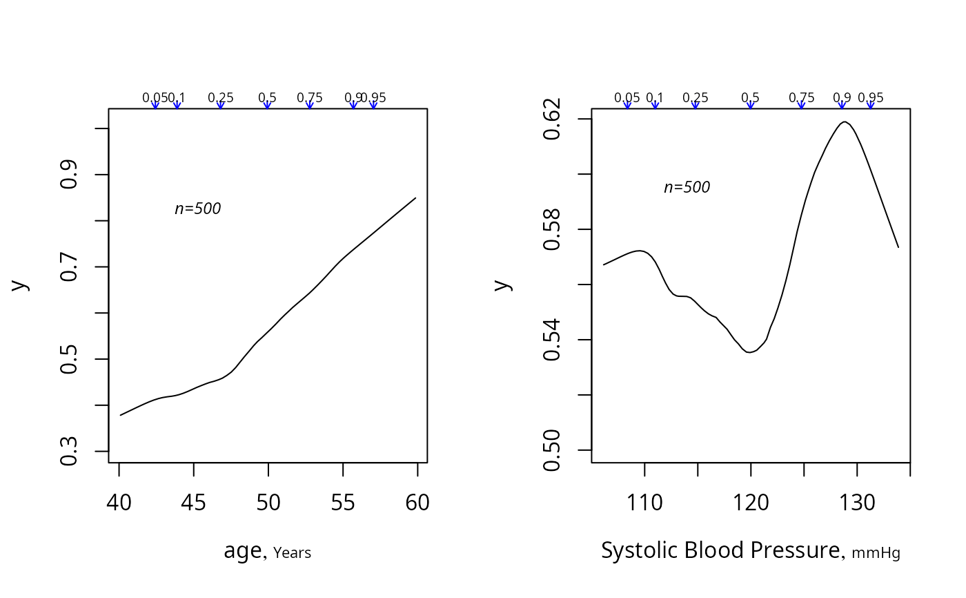
par(mfrow=c(1,2))
summaryRc(y ~ age + bp)

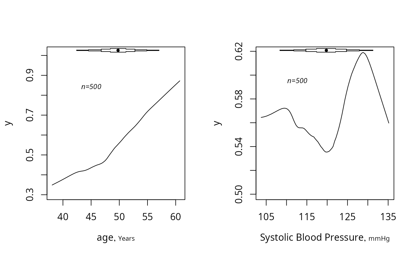
# For x limits use 1st and 99th percentiles to frame extended box plots
summaryRc(y ~ age + bp, bpplot='top', datadensity=FALSE, trim=.01)

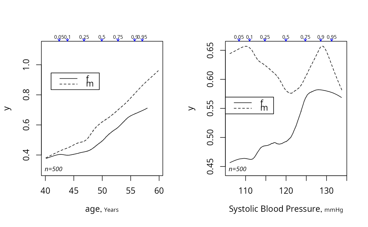
summaryRc(y ~ age + bp + stratify(sex),
          label.curves=list(keys='lines'), nloc=list(x=.1, y=.05))

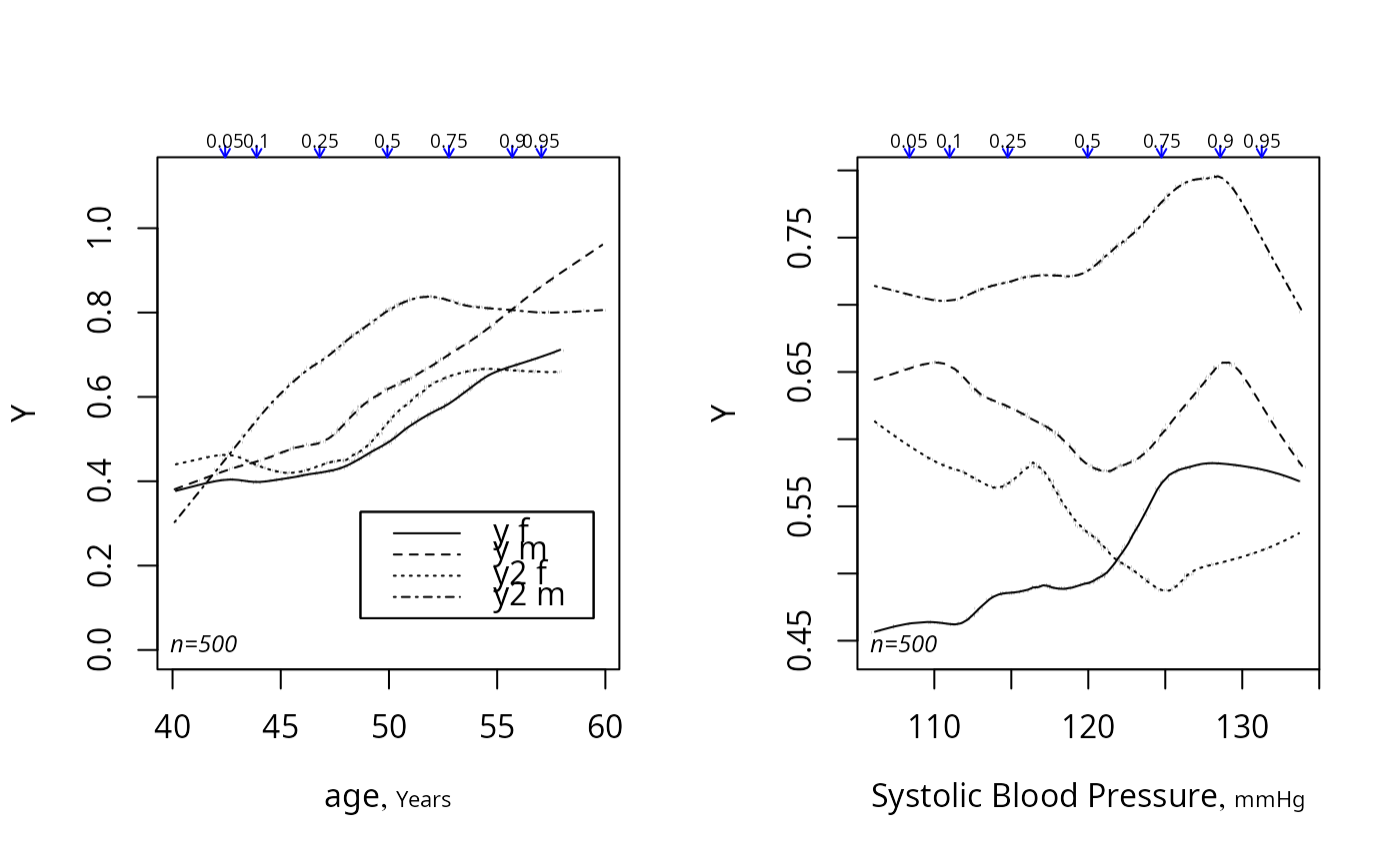
y2 <- rbinom(500, 1, plogis(L + .5))
Y <- cbind(y, y2)
summaryRc(Y ~ age + bp + stratify(sex),
          label.curves=list(keys='lines'), nloc=list(x=.1, y=.05))
#> Warning: no empty rectangle was large enough

#> No empty area large enough for automatic key positioning.  Specify keyloc or cex.
#> Width and height of key as computed by key(), in data units: 15.113  0.079