Data and Examples from Baltagi (2002)
Baltagi2002.RdThis manual page collects a list of examples from the book. Some solutions might not be exact and the list is certainly not complete. If you have suggestions for improvement (preferably in the form of code), please contact the package maintainer.
Examples
#> Loading required namespace: tseries
#> Registered S3 method overwritten by 'quantmod':
#> method from
#> as.zoo.data.frame zoo
#> Loading required namespace: strucchange
#> Loading required namespace: plm
#> Loading required namespace: systemfit
################################
## Cigarette consumption data ##
################################
## data
data("CigarettesB", package = "AER")
## Table 3.3
cig_lm <- lm(packs ~ price, data = CigarettesB)
summary(cig_lm)
#>
#> Call:
#> lm(formula = packs ~ price, data = CigarettesB)
#>
#> Residuals:
#> Min 1Q Median 3Q Max
#> -0.45472 -0.09968 0.00612 0.11553 0.29346
#>
#> Coefficients:
#> Estimate Std. Error t value Pr(>|t|)
#> (Intercept) 5.0941 0.0627 81.247 < 2e-16 ***
#> price -1.1983 0.2818 -4.253 0.000108 ***
#> ---
#> Signif. codes: 0 ‘***’ 0.001 ‘**’ 0.01 ‘*’ 0.05 ‘.’ 0.1 ‘ ’ 1
#>
#> Residual standard error: 0.163 on 44 degrees of freedom
#> Multiple R-squared: 0.2913, Adjusted R-squared: 0.2752
#> F-statistic: 18.08 on 1 and 44 DF, p-value: 0.0001085
#>
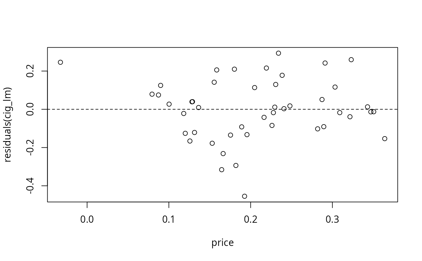
## Figure 3.9
plot(residuals(cig_lm) ~ price, data = CigarettesB)
abline(h = 0, lty = 2)
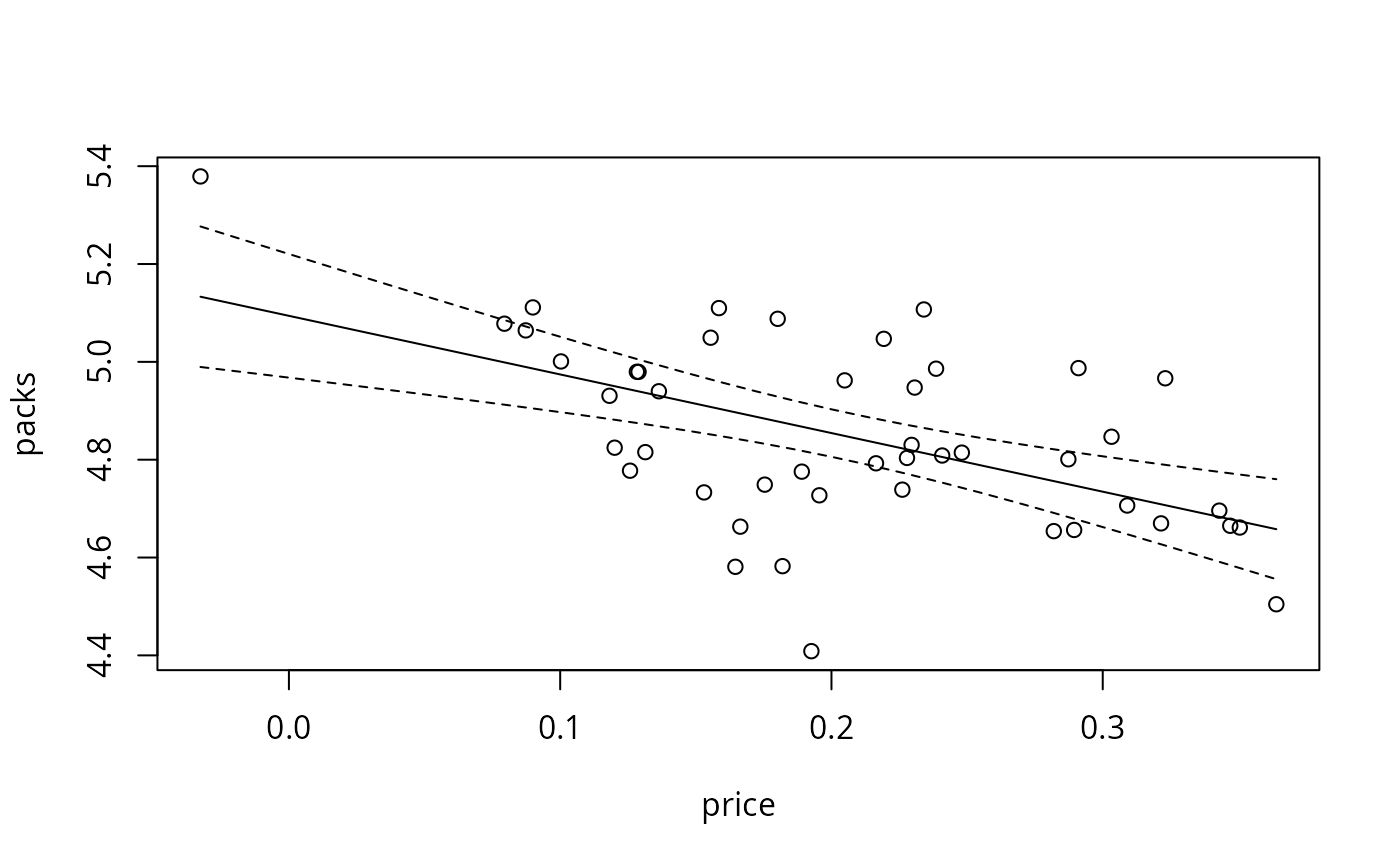
 ## Figure 3.10
cig_pred <- with(CigarettesB,
data.frame(price = seq(from = min(price), to = max(price), length = 30)))
cig_pred <- cbind(cig_pred, predict(cig_lm, newdata = cig_pred, interval = "confidence"))
plot(packs ~ price, data = CigarettesB)
lines(fit ~ price, data = cig_pred)
lines(lwr ~ price, data = cig_pred, lty = 2)
lines(upr ~ price, data = cig_pred, lty = 2)
## Figure 3.10
cig_pred <- with(CigarettesB,
data.frame(price = seq(from = min(price), to = max(price), length = 30)))
cig_pred <- cbind(cig_pred, predict(cig_lm, newdata = cig_pred, interval = "confidence"))
plot(packs ~ price, data = CigarettesB)
lines(fit ~ price, data = cig_pred)
lines(lwr ~ price, data = cig_pred, lty = 2)
lines(upr ~ price, data = cig_pred, lty = 2)
 ## Chapter 5: diagnostic tests (p. 111-115)
cig_lm2 <- lm(packs ~ price + income, data = CigarettesB)
summary(cig_lm2)
#>
#> Call:
#> lm(formula = packs ~ price + income, data = CigarettesB)
#>
#> Residuals:
#> Min 1Q Median 3Q Max
#> -0.41867 -0.10683 0.00757 0.11738 0.32868
#>
#> Coefficients:
#> Estimate Std. Error t value Pr(>|t|)
#> (Intercept) 4.2997 0.9089 4.730 2.43e-05 ***
#> price -1.3383 0.3246 -4.123 0.000168 ***
#> income 0.1724 0.1968 0.876 0.385818
#> ---
#> Signif. codes: 0 ‘***’ 0.001 ‘**’ 0.01 ‘*’ 0.05 ‘.’ 0.1 ‘ ’ 1
#>
#> Residual standard error: 0.1634 on 43 degrees of freedom
#> Multiple R-squared: 0.3037, Adjusted R-squared: 0.2713
#> F-statistic: 9.378 on 2 and 43 DF, p-value: 0.0004168
#>
## Glejser tests (p. 112)
ares <- abs(residuals(cig_lm2))
summary(lm(ares ~ income, data = CigarettesB))
#>
#> Call:
#> lm(formula = ares ~ income, data = CigarettesB)
#>
#> Residuals:
#> Min 1Q Median 3Q Max
#> -0.13738 -0.07061 -0.01891 0.07253 0.24508
#>
#> Coefficients:
#> Estimate Std. Error t value Pr(>|t|)
#> (Intercept) 1.16169 0.46267 2.511 0.0158 *
#> income -0.21689 0.09684 -2.240 0.0302 *
#> ---
#> Signif. codes: 0 ‘***’ 0.001 ‘**’ 0.01 ‘*’ 0.05 ‘.’ 0.1 ‘ ’ 1
#>
#> Residual standard error: 0.09242 on 44 degrees of freedom
#> Multiple R-squared: 0.1023, Adjusted R-squared: 0.08193
#> F-statistic: 5.016 on 1 and 44 DF, p-value: 0.03022
#>
summary(lm(ares ~ I(1/income), data = CigarettesB))
#>
#> Call:
#> lm(formula = ares ~ I(1/income), data = CigarettesB)
#>
#> Residuals:
#> Min 1Q Median 3Q Max
#> -0.14143 -0.07235 -0.01921 0.07227 0.24186
#>
#> Coefficients:
#> Estimate Std. Error t value Pr(>|t|)
#> (Intercept) -0.9489 0.4671 -2.032 0.0483 *
#> I(1/income) 5.1287 2.2277 2.302 0.0261 *
#> ---
#> Signif. codes: 0 ‘***’ 0.001 ‘**’ 0.01 ‘*’ 0.05 ‘.’ 0.1 ‘ ’ 1
#>
#> Residual standard error: 0.09215 on 44 degrees of freedom
#> Multiple R-squared: 0.1075, Adjusted R-squared: 0.08722
#> F-statistic: 5.3 on 1 and 44 DF, p-value: 0.02611
#>
summary(lm(ares ~ I(1/sqrt(income)), data = CigarettesB))
#>
#> Call:
#> lm(formula = ares ~ I(1/sqrt(income)), data = CigarettesB)
#>
#> Residuals:
#> Min 1Q Median 3Q Max
#> -0.14041 -0.07192 -0.01914 0.07233 0.24267
#>
#> Coefficients:
#> Estimate Std. Error t value Pr(>|t|)
#> (Intercept) -2.0045 0.9317 -2.151 0.0370 *
#> I(1/sqrt(income)) 4.6541 2.0352 2.287 0.0271 *
#> ---
#> Signif. codes: 0 ‘***’ 0.001 ‘**’ 0.01 ‘*’ 0.05 ‘.’ 0.1 ‘ ’ 1
#>
#> Residual standard error: 0.09222 on 44 degrees of freedom
#> Multiple R-squared: 0.1062, Adjusted R-squared: 0.08591
#> F-statistic: 5.229 on 1 and 44 DF, p-value: 0.02708
#>
summary(lm(ares ~ sqrt(income), data = CigarettesB))
#>
#> Call:
#> lm(formula = ares ~ sqrt(income), data = CigarettesB)
#>
#> Residuals:
#> Min 1Q Median 3Q Max
#> -0.13838 -0.07105 -0.01899 0.07247 0.24428
#>
#> Coefficients:
#> Estimate Std. Error t value Pr(>|t|)
#> (Intercept) 2.2172 0.9273 2.391 0.0211 *
#> sqrt(income) -0.9571 0.4243 -2.255 0.0291 *
#> ---
#> Signif. codes: 0 ‘***’ 0.001 ‘**’ 0.01 ‘*’ 0.05 ‘.’ 0.1 ‘ ’ 1
#>
#> Residual standard error: 0.09235 on 44 degrees of freedom
#> Multiple R-squared: 0.1036, Adjusted R-squared: 0.08326
#> F-statistic: 5.087 on 1 and 44 DF, p-value: 0.02913
#>
## Goldfeld-Quandt test (p. 112)
gqtest(cig_lm2, order.by = ~ income, data = CigarettesB, fraction = 12, alternative = "less")
#>
#> Goldfeld-Quandt test
#>
#> data: cig_lm2
#> GQ = 0.31846, df1 = 14, df2 = 14, p-value = 0.02017
#> alternative hypothesis: variance decreases from segment 1 to 2
#>
## NOTE: Baltagi computes the test statistic as mss1/mss2,
## i.e., tries to find decreasing variances. gqtest() always uses
## mss2/mss1 and has an "alternative" argument.
## Spearman rank correlation test (p. 113)
cor.test(~ ares + income, data = CigarettesB, method = "spearman")
#>
#> Spearman's rank correlation rho
#>
#> data: ares and income
#> S = 20784, p-value = 0.05813
#> alternative hypothesis: true rho is not equal to 0
#> sample estimates:
#> rho
#> -0.2817761
#>
## Breusch-Pagan test (p. 113)
bptest(cig_lm2, varformula = ~ income, data = CigarettesB, student = FALSE)
#>
#> Breusch-Pagan test
#>
#> data: cig_lm2
#> BP = 5.4852, df = 1, p-value = 0.01918
#>
## White test (Table 5.1, p. 113)
bptest(cig_lm2, ~ income * price + I(income^2) + I(price^2), data = CigarettesB)
#>
#> studentized Breusch-Pagan test
#>
#> data: cig_lm2
#> BP = 15.656, df = 5, p-value = 0.007897
#>
## White HC standard errors (Table 5.2, p. 114)
coeftest(cig_lm2, vcov = vcovHC(cig_lm2, type = "HC1"))
#>
#> t test of coefficients:
#>
#> Estimate Std. Error t value Pr(>|t|)
#> (Intercept) 4.29966 1.09523 3.9258 0.0003076 ***
#> price -1.33833 0.34337 -3.8977 0.0003352 ***
#> income 0.17239 0.23661 0.7286 0.4702172
#> ---
#> Signif. codes: 0 ‘***’ 0.001 ‘**’ 0.01 ‘*’ 0.05 ‘.’ 0.1 ‘ ’ 1
#>
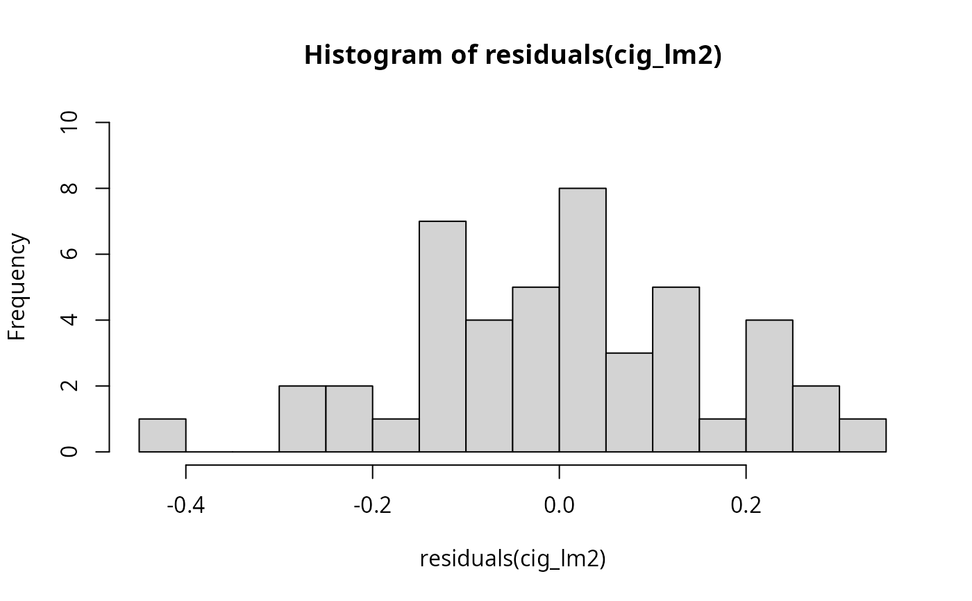
## Jarque-Bera test (Figure 5.2, p. 115)
hist(residuals(cig_lm2), breaks = 16, ylim = c(0, 10), col = "lightgray")
## Chapter 5: diagnostic tests (p. 111-115)
cig_lm2 <- lm(packs ~ price + income, data = CigarettesB)
summary(cig_lm2)
#>
#> Call:
#> lm(formula = packs ~ price + income, data = CigarettesB)
#>
#> Residuals:
#> Min 1Q Median 3Q Max
#> -0.41867 -0.10683 0.00757 0.11738 0.32868
#>
#> Coefficients:
#> Estimate Std. Error t value Pr(>|t|)
#> (Intercept) 4.2997 0.9089 4.730 2.43e-05 ***
#> price -1.3383 0.3246 -4.123 0.000168 ***
#> income 0.1724 0.1968 0.876 0.385818
#> ---
#> Signif. codes: 0 ‘***’ 0.001 ‘**’ 0.01 ‘*’ 0.05 ‘.’ 0.1 ‘ ’ 1
#>
#> Residual standard error: 0.1634 on 43 degrees of freedom
#> Multiple R-squared: 0.3037, Adjusted R-squared: 0.2713
#> F-statistic: 9.378 on 2 and 43 DF, p-value: 0.0004168
#>
## Glejser tests (p. 112)
ares <- abs(residuals(cig_lm2))
summary(lm(ares ~ income, data = CigarettesB))
#>
#> Call:
#> lm(formula = ares ~ income, data = CigarettesB)
#>
#> Residuals:
#> Min 1Q Median 3Q Max
#> -0.13738 -0.07061 -0.01891 0.07253 0.24508
#>
#> Coefficients:
#> Estimate Std. Error t value Pr(>|t|)
#> (Intercept) 1.16169 0.46267 2.511 0.0158 *
#> income -0.21689 0.09684 -2.240 0.0302 *
#> ---
#> Signif. codes: 0 ‘***’ 0.001 ‘**’ 0.01 ‘*’ 0.05 ‘.’ 0.1 ‘ ’ 1
#>
#> Residual standard error: 0.09242 on 44 degrees of freedom
#> Multiple R-squared: 0.1023, Adjusted R-squared: 0.08193
#> F-statistic: 5.016 on 1 and 44 DF, p-value: 0.03022
#>
summary(lm(ares ~ I(1/income), data = CigarettesB))
#>
#> Call:
#> lm(formula = ares ~ I(1/income), data = CigarettesB)
#>
#> Residuals:
#> Min 1Q Median 3Q Max
#> -0.14143 -0.07235 -0.01921 0.07227 0.24186
#>
#> Coefficients:
#> Estimate Std. Error t value Pr(>|t|)
#> (Intercept) -0.9489 0.4671 -2.032 0.0483 *
#> I(1/income) 5.1287 2.2277 2.302 0.0261 *
#> ---
#> Signif. codes: 0 ‘***’ 0.001 ‘**’ 0.01 ‘*’ 0.05 ‘.’ 0.1 ‘ ’ 1
#>
#> Residual standard error: 0.09215 on 44 degrees of freedom
#> Multiple R-squared: 0.1075, Adjusted R-squared: 0.08722
#> F-statistic: 5.3 on 1 and 44 DF, p-value: 0.02611
#>
summary(lm(ares ~ I(1/sqrt(income)), data = CigarettesB))
#>
#> Call:
#> lm(formula = ares ~ I(1/sqrt(income)), data = CigarettesB)
#>
#> Residuals:
#> Min 1Q Median 3Q Max
#> -0.14041 -0.07192 -0.01914 0.07233 0.24267
#>
#> Coefficients:
#> Estimate Std. Error t value Pr(>|t|)
#> (Intercept) -2.0045 0.9317 -2.151 0.0370 *
#> I(1/sqrt(income)) 4.6541 2.0352 2.287 0.0271 *
#> ---
#> Signif. codes: 0 ‘***’ 0.001 ‘**’ 0.01 ‘*’ 0.05 ‘.’ 0.1 ‘ ’ 1
#>
#> Residual standard error: 0.09222 on 44 degrees of freedom
#> Multiple R-squared: 0.1062, Adjusted R-squared: 0.08591
#> F-statistic: 5.229 on 1 and 44 DF, p-value: 0.02708
#>
summary(lm(ares ~ sqrt(income), data = CigarettesB))
#>
#> Call:
#> lm(formula = ares ~ sqrt(income), data = CigarettesB)
#>
#> Residuals:
#> Min 1Q Median 3Q Max
#> -0.13838 -0.07105 -0.01899 0.07247 0.24428
#>
#> Coefficients:
#> Estimate Std. Error t value Pr(>|t|)
#> (Intercept) 2.2172 0.9273 2.391 0.0211 *
#> sqrt(income) -0.9571 0.4243 -2.255 0.0291 *
#> ---
#> Signif. codes: 0 ‘***’ 0.001 ‘**’ 0.01 ‘*’ 0.05 ‘.’ 0.1 ‘ ’ 1
#>
#> Residual standard error: 0.09235 on 44 degrees of freedom
#> Multiple R-squared: 0.1036, Adjusted R-squared: 0.08326
#> F-statistic: 5.087 on 1 and 44 DF, p-value: 0.02913
#>
## Goldfeld-Quandt test (p. 112)
gqtest(cig_lm2, order.by = ~ income, data = CigarettesB, fraction = 12, alternative = "less")
#>
#> Goldfeld-Quandt test
#>
#> data: cig_lm2
#> GQ = 0.31846, df1 = 14, df2 = 14, p-value = 0.02017
#> alternative hypothesis: variance decreases from segment 1 to 2
#>
## NOTE: Baltagi computes the test statistic as mss1/mss2,
## i.e., tries to find decreasing variances. gqtest() always uses
## mss2/mss1 and has an "alternative" argument.
## Spearman rank correlation test (p. 113)
cor.test(~ ares + income, data = CigarettesB, method = "spearman")
#>
#> Spearman's rank correlation rho
#>
#> data: ares and income
#> S = 20784, p-value = 0.05813
#> alternative hypothesis: true rho is not equal to 0
#> sample estimates:
#> rho
#> -0.2817761
#>
## Breusch-Pagan test (p. 113)
bptest(cig_lm2, varformula = ~ income, data = CigarettesB, student = FALSE)
#>
#> Breusch-Pagan test
#>
#> data: cig_lm2
#> BP = 5.4852, df = 1, p-value = 0.01918
#>
## White test (Table 5.1, p. 113)
bptest(cig_lm2, ~ income * price + I(income^2) + I(price^2), data = CigarettesB)
#>
#> studentized Breusch-Pagan test
#>
#> data: cig_lm2
#> BP = 15.656, df = 5, p-value = 0.007897
#>
## White HC standard errors (Table 5.2, p. 114)
coeftest(cig_lm2, vcov = vcovHC(cig_lm2, type = "HC1"))
#>
#> t test of coefficients:
#>
#> Estimate Std. Error t value Pr(>|t|)
#> (Intercept) 4.29966 1.09523 3.9258 0.0003076 ***
#> price -1.33833 0.34337 -3.8977 0.0003352 ***
#> income 0.17239 0.23661 0.7286 0.4702172
#> ---
#> Signif. codes: 0 ‘***’ 0.001 ‘**’ 0.01 ‘*’ 0.05 ‘.’ 0.1 ‘ ’ 1
#>
## Jarque-Bera test (Figure 5.2, p. 115)
hist(residuals(cig_lm2), breaks = 16, ylim = c(0, 10), col = "lightgray")
 library("tseries")
jarque.bera.test(residuals(cig_lm2))
#>
#> Jarque Bera Test
#>
#> data: residuals(cig_lm2)
#> X-squared = 0.28935, df = 2, p-value = 0.8653
#>
## Tables 8.1 and 8.2
influence.measures(cig_lm2)
#> Influence measures of
#> lm(formula = packs ~ price + income, data = CigarettesB) :
#>
#> dfb.1_ dfb.pric dfb.incm dffit cov.r cook.d hat inf
#> AL 0.14503 0.069010 -0.14188 0.19186 1.070 1.23e-02 0.0480
#> AZ -0.11311 0.033072 0.10173 -0.25077 0.968 2.05e-02 0.0315
#> AR 0.56419 0.376064 -0.56381 0.66702 0.847 1.36e-01 0.0847
#> CA -0.01386 -0.255192 0.02769 -0.31637 1.114 3.34e-02 0.0975
#> CT 0.15244 -0.022453 -0.14793 -0.20087 1.219 1.37e-02 0.1354 *
#> DE -0.12654 -0.037389 0.12991 0.23129 0.992 1.76e-02 0.0326
#> DC 0.23239 0.001472 -0.22823 -0.29167 1.149 2.86e-02 0.1104
#> FL 0.01116 0.050233 -0.01301 0.07389 1.112 1.86e-03 0.0431
#> GA -0.00269 -0.028971 0.00551 0.04527 1.114 6.99e-04 0.0402
#> ID -0.10101 -0.013791 0.09591 -0.15005 1.079 7.59e-03 0.0413
#> IL -0.00101 0.000075 0.00101 0.00178 1.118 1.09e-06 0.0399
#> IN -0.03076 -0.153574 0.04353 0.19363 1.105 1.26e-02 0.0650
#> IA 0.00638 0.007696 -0.00639 0.01509 1.107 7.77e-05 0.0310
#> KS 0.00314 -0.002575 -0.00389 -0.04083 1.092 5.68e-04 0.0223
#> KY -0.09222 -0.725107 0.14758 0.80979 1.113 2.10e-01 0.1977 *
#> LA 0.31705 0.226157 -0.31744 0.38745 1.022 4.91e-02 0.0761
#> ME 0.17424 0.309538 -0.18410 0.40000 0.940 5.13e-02 0.0553
#> MD 0.39398 0.378023 -0.41346 -0.50701 1.073 8.40e-02 0.1216
#> MA 0.19840 0.073723 -0.20018 -0.23411 1.126 1.84e-02 0.0856
#> MI -0.00898 0.025355 0.00991 0.12316 1.052 5.10e-03 0.0238
#> MN 0.01342 0.042769 -0.01537 0.05001 1.172 8.53e-04 0.0864
#> MS 0.06675 0.002382 -0.06369 0.08277 1.171 2.33e-03 0.0883
#> MO -0.03986 -0.089643 0.04634 0.10541 1.154 3.78e-03 0.0787
#> MT -0.04820 0.067706 0.03769 -0.19283 1.021 1.24e-02 0.0312
#> NE 0.02185 0.027580 -0.02540 -0.09498 1.072 3.05e-03 0.0243
#> NV 0.05366 0.347879 -0.06990 0.45042 0.937 6.47e-02 0.0646
#> NH -0.34967 -0.257318 0.36079 0.40764 1.142 5.53e-02 0.1308
#> NJ 0.12527 -0.004859 -0.12241 -0.15616 1.234 8.29e-03 0.1394 *
#> NM -0.38923 -0.064661 0.37379 -0.49010 0.901 7.56e-02 0.0639
#> NY 0.01626 -0.028925 -0.01431 -0.05033 1.175 8.64e-04 0.0888
#> ND -0.15387 -0.005358 0.14232 -0.31360 0.885 3.12e-02 0.0295
#> OH -0.00856 -0.028773 0.01108 0.04159 1.117 5.90e-04 0.0423
#> OK -0.12028 -0.047228 0.11708 -0.15599 1.094 8.21e-03 0.0505
#> PA 0.00741 -0.001370 -0.00765 -0.02452 1.100 2.05e-04 0.0257
#> RI 0.00218 0.114469 -0.00738 0.16917 1.088 9.64e-03 0.0504
#> SC 0.04282 -0.092254 -0.03271 0.15382 1.132 8.02e-03 0.0725
#> SD -0.04178 0.064802 0.03307 -0.14581 1.079 7.17e-03 0.0402
#> TN 0.01884 -0.062711 -0.01037 0.15431 1.046 7.98e-03 0.0294
#> TX -0.06472 -0.095510 0.06734 -0.12671 1.113 5.44e-03 0.0546
#> UT -0.77803 -0.317059 0.76368 -0.88760 0.679 2.24e-01 0.0856 *
#> VT -0.02396 -0.065794 0.03278 0.20305 0.979 1.35e-02 0.0243
#> VA 0.05235 0.069110 -0.05673 -0.08713 1.156 2.59e-03 0.0773
#> WA -0.00136 -0.010137 0.00187 -0.01242 1.175 5.27e-05 0.0866
#> WV -0.11903 0.031391 0.11039 -0.17766 1.122 1.07e-02 0.0709
#> WI 0.00494 0.006306 -0.00481 0.01736 1.100 1.03e-04 0.0254
#> WY -0.00156 -0.025435 0.00388 0.03501 1.135 4.18e-04 0.0555
#####################################
## US consumption data (1950-1993) ##
#####################################
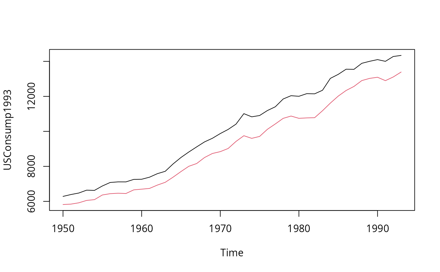
## data
data("USConsump1993", package = "AER")
plot(USConsump1993, plot.type = "single", col = 1:2)
library("tseries")
jarque.bera.test(residuals(cig_lm2))
#>
#> Jarque Bera Test
#>
#> data: residuals(cig_lm2)
#> X-squared = 0.28935, df = 2, p-value = 0.8653
#>
## Tables 8.1 and 8.2
influence.measures(cig_lm2)
#> Influence measures of
#> lm(formula = packs ~ price + income, data = CigarettesB) :
#>
#> dfb.1_ dfb.pric dfb.incm dffit cov.r cook.d hat inf
#> AL 0.14503 0.069010 -0.14188 0.19186 1.070 1.23e-02 0.0480
#> AZ -0.11311 0.033072 0.10173 -0.25077 0.968 2.05e-02 0.0315
#> AR 0.56419 0.376064 -0.56381 0.66702 0.847 1.36e-01 0.0847
#> CA -0.01386 -0.255192 0.02769 -0.31637 1.114 3.34e-02 0.0975
#> CT 0.15244 -0.022453 -0.14793 -0.20087 1.219 1.37e-02 0.1354 *
#> DE -0.12654 -0.037389 0.12991 0.23129 0.992 1.76e-02 0.0326
#> DC 0.23239 0.001472 -0.22823 -0.29167 1.149 2.86e-02 0.1104
#> FL 0.01116 0.050233 -0.01301 0.07389 1.112 1.86e-03 0.0431
#> GA -0.00269 -0.028971 0.00551 0.04527 1.114 6.99e-04 0.0402
#> ID -0.10101 -0.013791 0.09591 -0.15005 1.079 7.59e-03 0.0413
#> IL -0.00101 0.000075 0.00101 0.00178 1.118 1.09e-06 0.0399
#> IN -0.03076 -0.153574 0.04353 0.19363 1.105 1.26e-02 0.0650
#> IA 0.00638 0.007696 -0.00639 0.01509 1.107 7.77e-05 0.0310
#> KS 0.00314 -0.002575 -0.00389 -0.04083 1.092 5.68e-04 0.0223
#> KY -0.09222 -0.725107 0.14758 0.80979 1.113 2.10e-01 0.1977 *
#> LA 0.31705 0.226157 -0.31744 0.38745 1.022 4.91e-02 0.0761
#> ME 0.17424 0.309538 -0.18410 0.40000 0.940 5.13e-02 0.0553
#> MD 0.39398 0.378023 -0.41346 -0.50701 1.073 8.40e-02 0.1216
#> MA 0.19840 0.073723 -0.20018 -0.23411 1.126 1.84e-02 0.0856
#> MI -0.00898 0.025355 0.00991 0.12316 1.052 5.10e-03 0.0238
#> MN 0.01342 0.042769 -0.01537 0.05001 1.172 8.53e-04 0.0864
#> MS 0.06675 0.002382 -0.06369 0.08277 1.171 2.33e-03 0.0883
#> MO -0.03986 -0.089643 0.04634 0.10541 1.154 3.78e-03 0.0787
#> MT -0.04820 0.067706 0.03769 -0.19283 1.021 1.24e-02 0.0312
#> NE 0.02185 0.027580 -0.02540 -0.09498 1.072 3.05e-03 0.0243
#> NV 0.05366 0.347879 -0.06990 0.45042 0.937 6.47e-02 0.0646
#> NH -0.34967 -0.257318 0.36079 0.40764 1.142 5.53e-02 0.1308
#> NJ 0.12527 -0.004859 -0.12241 -0.15616 1.234 8.29e-03 0.1394 *
#> NM -0.38923 -0.064661 0.37379 -0.49010 0.901 7.56e-02 0.0639
#> NY 0.01626 -0.028925 -0.01431 -0.05033 1.175 8.64e-04 0.0888
#> ND -0.15387 -0.005358 0.14232 -0.31360 0.885 3.12e-02 0.0295
#> OH -0.00856 -0.028773 0.01108 0.04159 1.117 5.90e-04 0.0423
#> OK -0.12028 -0.047228 0.11708 -0.15599 1.094 8.21e-03 0.0505
#> PA 0.00741 -0.001370 -0.00765 -0.02452 1.100 2.05e-04 0.0257
#> RI 0.00218 0.114469 -0.00738 0.16917 1.088 9.64e-03 0.0504
#> SC 0.04282 -0.092254 -0.03271 0.15382 1.132 8.02e-03 0.0725
#> SD -0.04178 0.064802 0.03307 -0.14581 1.079 7.17e-03 0.0402
#> TN 0.01884 -0.062711 -0.01037 0.15431 1.046 7.98e-03 0.0294
#> TX -0.06472 -0.095510 0.06734 -0.12671 1.113 5.44e-03 0.0546
#> UT -0.77803 -0.317059 0.76368 -0.88760 0.679 2.24e-01 0.0856 *
#> VT -0.02396 -0.065794 0.03278 0.20305 0.979 1.35e-02 0.0243
#> VA 0.05235 0.069110 -0.05673 -0.08713 1.156 2.59e-03 0.0773
#> WA -0.00136 -0.010137 0.00187 -0.01242 1.175 5.27e-05 0.0866
#> WV -0.11903 0.031391 0.11039 -0.17766 1.122 1.07e-02 0.0709
#> WI 0.00494 0.006306 -0.00481 0.01736 1.100 1.03e-04 0.0254
#> WY -0.00156 -0.025435 0.00388 0.03501 1.135 4.18e-04 0.0555
#####################################
## US consumption data (1950-1993) ##
#####################################
## data
data("USConsump1993", package = "AER")
plot(USConsump1993, plot.type = "single", col = 1:2)
 ## Chapter 5 (p. 122-125)
fm <- lm(expenditure ~ income, data = USConsump1993)
summary(fm)
#>
#> Call:
#> lm(formula = expenditure ~ income, data = USConsump1993)
#>
#> Residuals:
#> Min 1Q Median 3Q Max
#> -294.52 -67.02 4.64 90.02 325.84
#>
#> Coefficients:
#> Estimate Std. Error t value Pr(>|t|)
#> (Intercept) -65.795821 90.990824 -0.723 0.474
#> income 0.915623 0.008648 105.874 <2e-16 ***
#> ---
#> Signif. codes: 0 ‘***’ 0.001 ‘**’ 0.01 ‘*’ 0.05 ‘.’ 0.1 ‘ ’ 1
#>
#> Residual standard error: 153.6 on 42 degrees of freedom
#> Multiple R-squared: 0.9963, Adjusted R-squared: 0.9962
#> F-statistic: 1.121e+04 on 1 and 42 DF, p-value: < 2.2e-16
#>
## Durbin-Watson test (p. 122)
dwtest(fm)
#>
#> Durbin-Watson test
#>
#> data: fm
#> DW = 0.46078, p-value = 3.274e-11
#> alternative hypothesis: true autocorrelation is greater than 0
#>
## Breusch-Godfrey test (Table 5.4, p. 124)
bgtest(fm)
#>
#> Breusch-Godfrey test for serial correlation of order up to 1
#>
#> data: fm
#> LM test = 24.901, df = 1, p-value = 6.034e-07
#>
## Newey-West standard errors (Table 5.5, p. 125)
coeftest(fm, vcov = NeweyWest(fm, lag = 3, prewhite = FALSE, adjust = TRUE))
#>
#> t test of coefficients:
#>
#> Estimate Std. Error t value Pr(>|t|)
#> (Intercept) -65.795821 133.345400 -0.4934 0.6243
#> income 0.915623 0.015458 59.2319 <2e-16 ***
#> ---
#> Signif. codes: 0 ‘***’ 0.001 ‘**’ 0.01 ‘*’ 0.05 ‘.’ 0.1 ‘ ’ 1
#>
## Chapter 8
library("strucchange")
## Recursive residuals
rr <- recresid(fm)
rr
#> [1] 24.900681 30.354827 50.893291 63.260389 -49.805907 -28.404311
#> [7] -31.520559 53.194256 67.696114 -2.646556 9.679147 39.658827
#> [13] -40.126557 -30.260756 2.605633 -78.941467 27.185066 64.363195
#> [19] -64.906717 -71.641013 70.095867 -113.475323 -85.633171 -29.427630
#> [25] 128.328459 220.693133 126.591749 78.394247 -25.955574 -124.178686
#> [31] -90.845193 127.830581 -30.794629 159.780872 201.707127 405.310561
#> [37] 390.953841 373.370919 316.431235 188.109683 134.461285 339.300414
## Recursive CUSUM test
rcus <- efp(expenditure ~ income, data = USConsump1993)
plot(rcus)
## Chapter 5 (p. 122-125)
fm <- lm(expenditure ~ income, data = USConsump1993)
summary(fm)
#>
#> Call:
#> lm(formula = expenditure ~ income, data = USConsump1993)
#>
#> Residuals:
#> Min 1Q Median 3Q Max
#> -294.52 -67.02 4.64 90.02 325.84
#>
#> Coefficients:
#> Estimate Std. Error t value Pr(>|t|)
#> (Intercept) -65.795821 90.990824 -0.723 0.474
#> income 0.915623 0.008648 105.874 <2e-16 ***
#> ---
#> Signif. codes: 0 ‘***’ 0.001 ‘**’ 0.01 ‘*’ 0.05 ‘.’ 0.1 ‘ ’ 1
#>
#> Residual standard error: 153.6 on 42 degrees of freedom
#> Multiple R-squared: 0.9963, Adjusted R-squared: 0.9962
#> F-statistic: 1.121e+04 on 1 and 42 DF, p-value: < 2.2e-16
#>
## Durbin-Watson test (p. 122)
dwtest(fm)
#>
#> Durbin-Watson test
#>
#> data: fm
#> DW = 0.46078, p-value = 3.274e-11
#> alternative hypothesis: true autocorrelation is greater than 0
#>
## Breusch-Godfrey test (Table 5.4, p. 124)
bgtest(fm)
#>
#> Breusch-Godfrey test for serial correlation of order up to 1
#>
#> data: fm
#> LM test = 24.901, df = 1, p-value = 6.034e-07
#>
## Newey-West standard errors (Table 5.5, p. 125)
coeftest(fm, vcov = NeweyWest(fm, lag = 3, prewhite = FALSE, adjust = TRUE))
#>
#> t test of coefficients:
#>
#> Estimate Std. Error t value Pr(>|t|)
#> (Intercept) -65.795821 133.345400 -0.4934 0.6243
#> income 0.915623 0.015458 59.2319 <2e-16 ***
#> ---
#> Signif. codes: 0 ‘***’ 0.001 ‘**’ 0.01 ‘*’ 0.05 ‘.’ 0.1 ‘ ’ 1
#>
## Chapter 8
library("strucchange")
## Recursive residuals
rr <- recresid(fm)
rr
#> [1] 24.900681 30.354827 50.893291 63.260389 -49.805907 -28.404311
#> [7] -31.520559 53.194256 67.696114 -2.646556 9.679147 39.658827
#> [13] -40.126557 -30.260756 2.605633 -78.941467 27.185066 64.363195
#> [19] -64.906717 -71.641013 70.095867 -113.475323 -85.633171 -29.427630
#> [25] 128.328459 220.693133 126.591749 78.394247 -25.955574 -124.178686
#> [31] -90.845193 127.830581 -30.794629 159.780872 201.707127 405.310561
#> [37] 390.953841 373.370919 316.431235 188.109683 134.461285 339.300414
## Recursive CUSUM test
rcus <- efp(expenditure ~ income, data = USConsump1993)
plot(rcus)
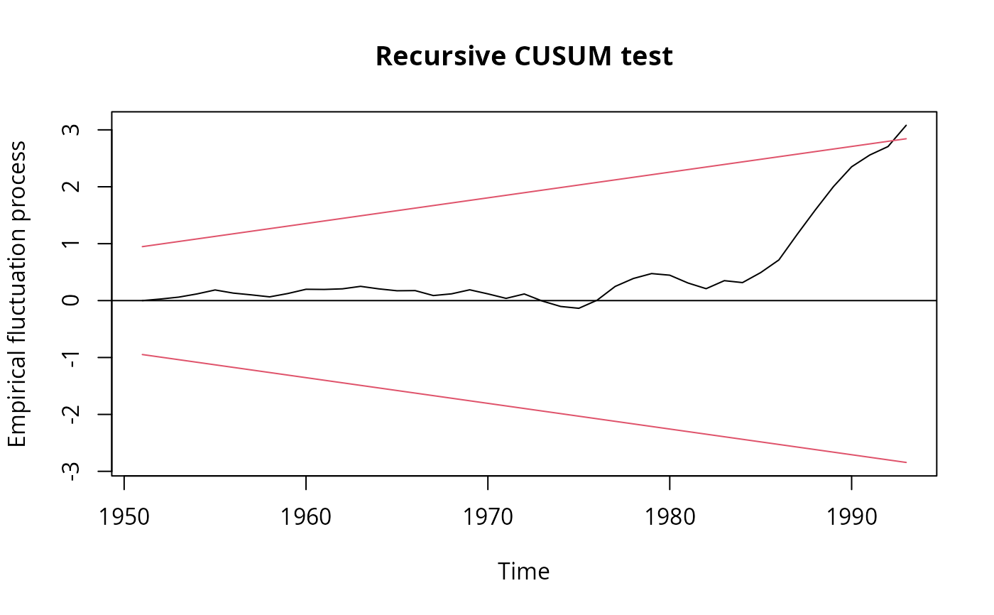 sctest(rcus)
#>
#> Recursive CUSUM test
#>
#> data: rcus
#> S = 1.0267, p-value = 0.02707
#>
## Harvey-Collier test
harvtest(fm)
#>
#> Harvey-Collier test
#>
#> data: fm
#> HC = 3.0802, df = 41, p-value = 0.003685
#>
## NOTE" Mistake in Baltagi (2002) who computes
## the t-statistic incorrectly as 0.0733 via
mean(rr)/sd(rr)/sqrt(length(rr))
#> [1] 0.07333754
## whereas it should be (as in harvtest)
mean(rr)/sd(rr) * sqrt(length(rr))
#> [1] 3.080177
## Rainbow test
raintest(fm, center = 23)
#>
#> Rainbow test
#>
#> data: fm
#> Rain = 4.1448, df1 = 22, df2 = 20, p-value = 0.001116
#>
## J test for non-nested models
library("dynlm")
fm1 <- dynlm(expenditure ~ income + L(income), data = USConsump1993)
fm2 <- dynlm(expenditure ~ income + L(expenditure), data = USConsump1993)
jtest(fm1, fm2)
#> J test
#>
#> Model 1: expenditure ~ income + L(income)
#> Model 2: expenditure ~ income + L(expenditure)
#> Estimate Std. Error t value Pr(>|t|)
#> M1 + fitted(M2) 1.6378 0.20984 7.8051 1.726e-09 ***
#> M2 + fitted(M1) -2.5419 0.61603 -4.1262 0.0001874 ***
#> ---
#> Signif. codes: 0 ‘***’ 0.001 ‘**’ 0.01 ‘*’ 0.05 ‘.’ 0.1 ‘ ’ 1
## Chapter 11
## Table 11.1 Instrumental-variables regression
usc <- as.data.frame(USConsump1993)
usc$investment <- usc$income - usc$expenditure
fm_ols <- lm(expenditure ~ income, data = usc)
fm_iv <- ivreg(expenditure ~ income | investment, data = usc)
## Hausman test
cf_diff <- coef(fm_iv) - coef(fm_ols)
vc_diff <- vcov(fm_iv) - vcov(fm_ols)
x2_diff <- as.vector(t(cf_diff) %*% solve(vc_diff) %*% cf_diff)
pchisq(x2_diff, df = 2, lower.tail = FALSE)
#> [1] 0.0001836953
## Chapter 14
## ACF and PACF for expenditures and first differences
exps <- USConsump1993[, "expenditure"]
(acf(exps))
sctest(rcus)
#>
#> Recursive CUSUM test
#>
#> data: rcus
#> S = 1.0267, p-value = 0.02707
#>
## Harvey-Collier test
harvtest(fm)
#>
#> Harvey-Collier test
#>
#> data: fm
#> HC = 3.0802, df = 41, p-value = 0.003685
#>
## NOTE" Mistake in Baltagi (2002) who computes
## the t-statistic incorrectly as 0.0733 via
mean(rr)/sd(rr)/sqrt(length(rr))
#> [1] 0.07333754
## whereas it should be (as in harvtest)
mean(rr)/sd(rr) * sqrt(length(rr))
#> [1] 3.080177
## Rainbow test
raintest(fm, center = 23)
#>
#> Rainbow test
#>
#> data: fm
#> Rain = 4.1448, df1 = 22, df2 = 20, p-value = 0.001116
#>
## J test for non-nested models
library("dynlm")
fm1 <- dynlm(expenditure ~ income + L(income), data = USConsump1993)
fm2 <- dynlm(expenditure ~ income + L(expenditure), data = USConsump1993)
jtest(fm1, fm2)
#> J test
#>
#> Model 1: expenditure ~ income + L(income)
#> Model 2: expenditure ~ income + L(expenditure)
#> Estimate Std. Error t value Pr(>|t|)
#> M1 + fitted(M2) 1.6378 0.20984 7.8051 1.726e-09 ***
#> M2 + fitted(M1) -2.5419 0.61603 -4.1262 0.0001874 ***
#> ---
#> Signif. codes: 0 ‘***’ 0.001 ‘**’ 0.01 ‘*’ 0.05 ‘.’ 0.1 ‘ ’ 1
## Chapter 11
## Table 11.1 Instrumental-variables regression
usc <- as.data.frame(USConsump1993)
usc$investment <- usc$income - usc$expenditure
fm_ols <- lm(expenditure ~ income, data = usc)
fm_iv <- ivreg(expenditure ~ income | investment, data = usc)
## Hausman test
cf_diff <- coef(fm_iv) - coef(fm_ols)
vc_diff <- vcov(fm_iv) - vcov(fm_ols)
x2_diff <- as.vector(t(cf_diff) %*% solve(vc_diff) %*% cf_diff)
pchisq(x2_diff, df = 2, lower.tail = FALSE)
#> [1] 0.0001836953
## Chapter 14
## ACF and PACF for expenditures and first differences
exps <- USConsump1993[, "expenditure"]
(acf(exps))
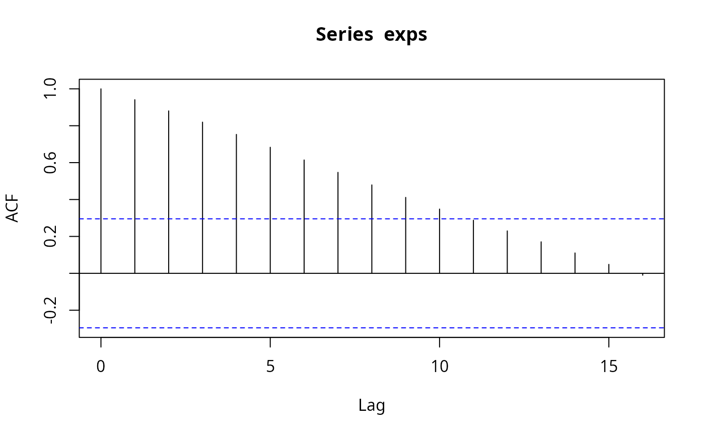 #>
#> Autocorrelations of series ‘exps’, by lag
#>
#> 0 1 2 3 4 5 6 7 8 9 10
#> 1.000 0.941 0.880 0.820 0.753 0.683 0.614 0.547 0.479 0.412 0.348
#> 11 12 13 14 15 16
#> 0.288 0.230 0.171 0.110 0.049 -0.010
(pacf(exps))
#>
#> Autocorrelations of series ‘exps’, by lag
#>
#> 0 1 2 3 4 5 6 7 8 9 10
#> 1.000 0.941 0.880 0.820 0.753 0.683 0.614 0.547 0.479 0.412 0.348
#> 11 12 13 14 15 16
#> 0.288 0.230 0.171 0.110 0.049 -0.010
(pacf(exps))
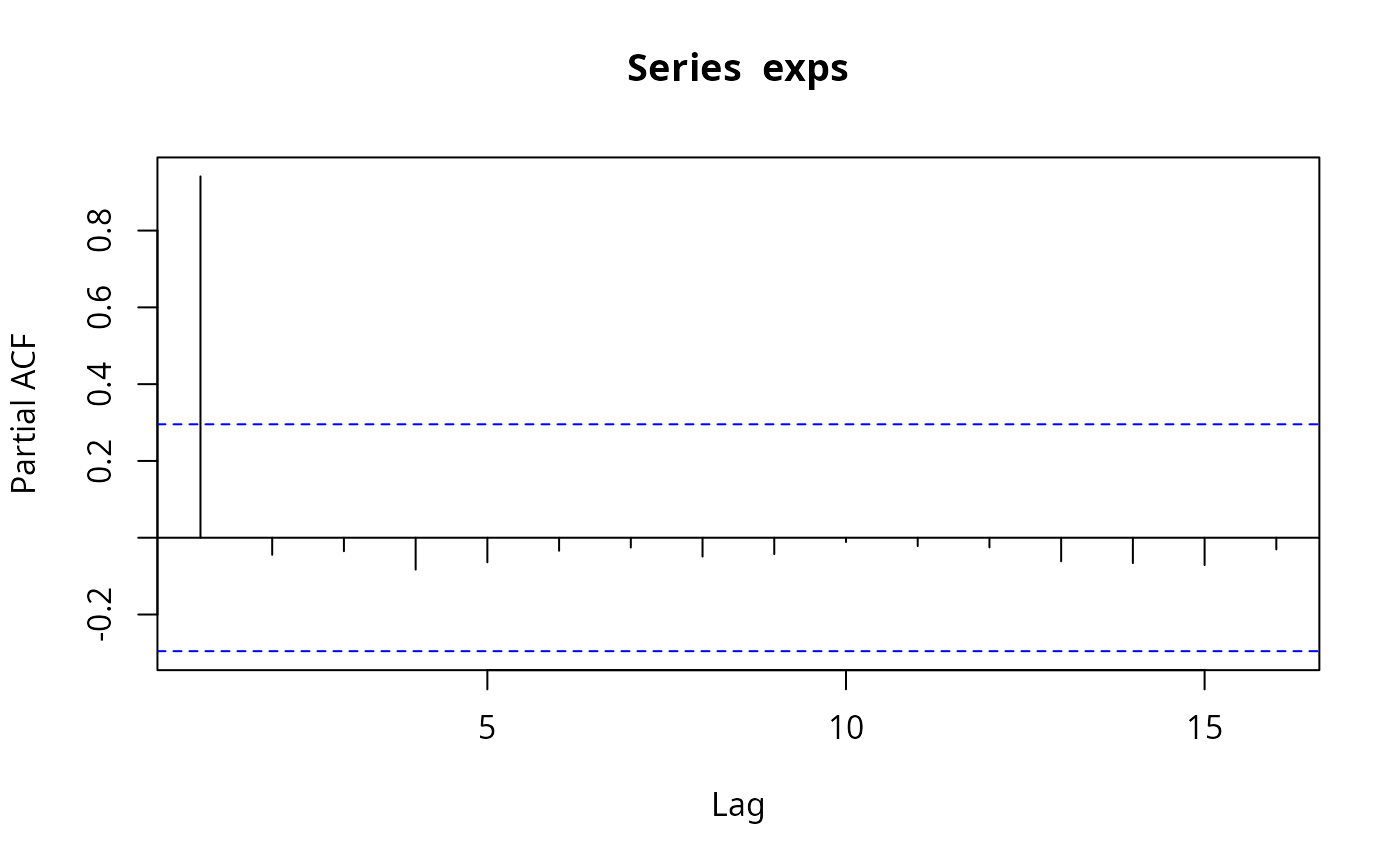 #>
#> Partial autocorrelations of series ‘exps’, by lag
#>
#> 1 2 3 4 5 6 7 8 9 10 11
#> 0.941 -0.045 -0.035 -0.083 -0.064 -0.034 -0.025 -0.049 -0.043 -0.011 -0.022
#> 12 13 14 15 16
#> -0.025 -0.061 -0.066 -0.071 -0.030
(acf(diff(exps)))
#>
#> Partial autocorrelations of series ‘exps’, by lag
#>
#> 1 2 3 4 5 6 7 8 9 10 11
#> 0.941 -0.045 -0.035 -0.083 -0.064 -0.034 -0.025 -0.049 -0.043 -0.011 -0.022
#> 12 13 14 15 16
#> -0.025 -0.061 -0.066 -0.071 -0.030
(acf(diff(exps)))
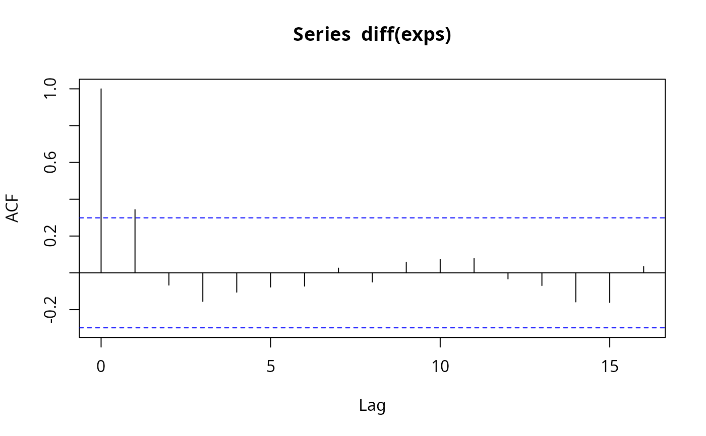 #>
#> Autocorrelations of series ‘diff(exps)’, by lag
#>
#> 0 1 2 3 4 5 6 7 8 9 10
#> 1.000 0.344 -0.067 -0.156 -0.105 -0.077 -0.072 0.026 -0.050 0.058 0.073
#> 11 12 13 14 15 16
#> 0.078 -0.033 -0.069 -0.158 -0.161 0.034
(pacf(diff(exps)))
#>
#> Autocorrelations of series ‘diff(exps)’, by lag
#>
#> 0 1 2 3 4 5 6 7 8 9 10
#> 1.000 0.344 -0.067 -0.156 -0.105 -0.077 -0.072 0.026 -0.050 0.058 0.073
#> 11 12 13 14 15 16
#> 0.078 -0.033 -0.069 -0.158 -0.161 0.034
(pacf(diff(exps)))
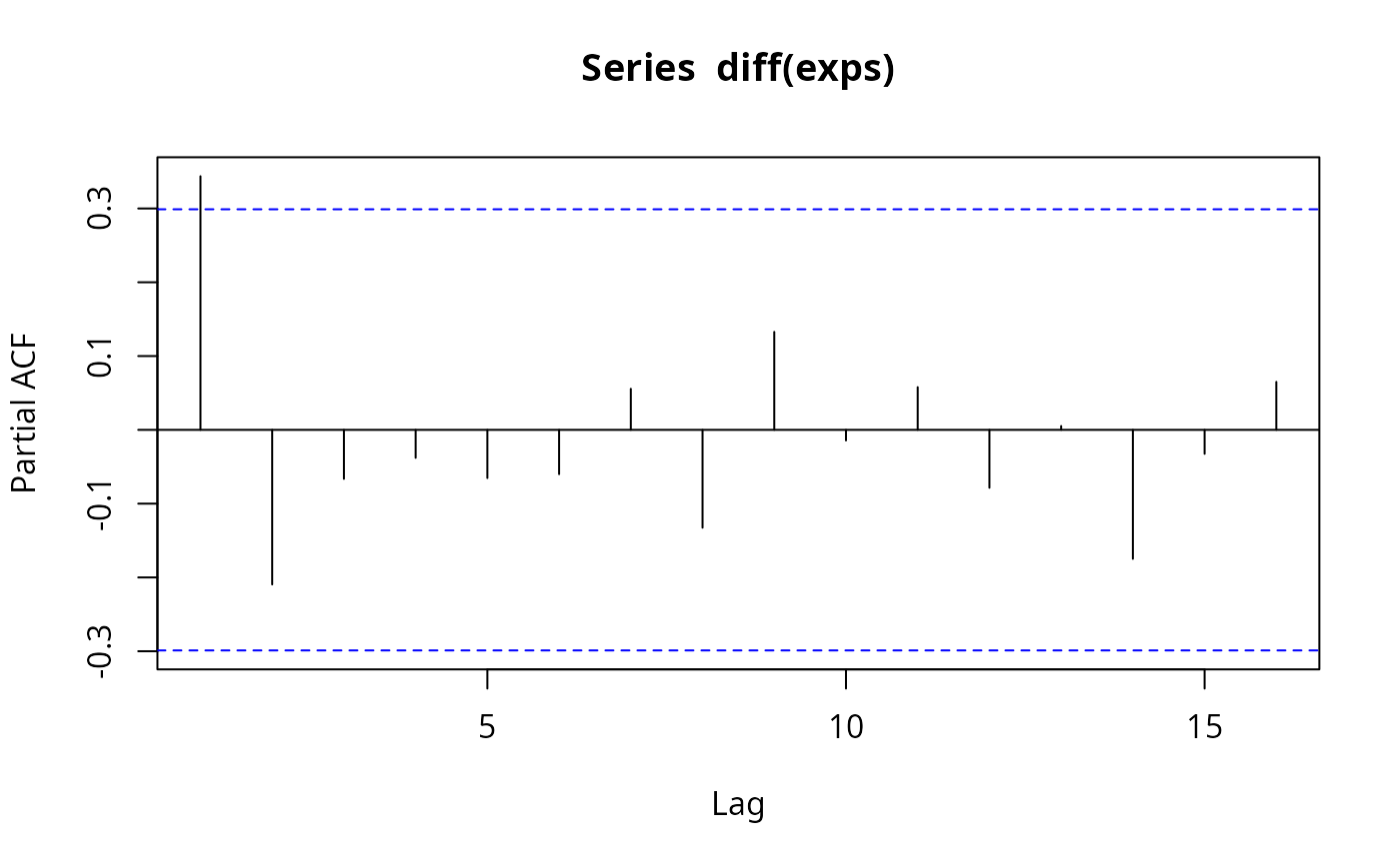 #>
#> Partial autocorrelations of series ‘diff(exps)’, by lag
#>
#> 1 2 3 4 5 6 7 8 9 10 11
#> 0.344 -0.209 -0.066 -0.038 -0.065 -0.060 0.056 -0.133 0.133 -0.014 0.058
#> 12 13 14 15 16
#> -0.079 0.005 -0.175 -0.032 0.065
## dynamic regressions, eq. (14.8)
fm <- dynlm(d(exps) ~ I(time(exps) - 1949) + L(exps))
summary(fm)
#>
#> Time series regression with "ts" data:
#> Start = 1951, End = 1993
#>
#> Call:
#> dynlm(formula = d(exps) ~ I(time(exps) - 1949) + L(exps))
#>
#> Residuals:
#> Min 1Q Median 3Q Max
#> -357.76 -78.18 22.49 108.97 201.06
#>
#> Coefficients:
#> Estimate Std. Error t value Pr(>|t|)
#> (Intercept) 1048.96039 353.81291 2.965 0.00509 **
#> I(time(exps) - 1949) 39.90164 14.31344 2.788 0.00808 **
#> L(exps) -0.19561 0.07398 -2.644 0.01164 *
#> ---
#> Signif. codes: 0 ‘***’ 0.001 ‘**’ 0.01 ‘*’ 0.05 ‘.’ 0.1 ‘ ’ 1
#>
#> Residual standard error: 147.4 on 40 degrees of freedom
#> Multiple R-squared: 0.1784, Adjusted R-squared: 0.1373
#> F-statistic: 4.343 on 2 and 40 DF, p-value: 0.01963
#>
################################
## Grunfeld's investment data ##
################################
## select the first three companies (as panel data)
data("Grunfeld", package = "AER")
pgr <- subset(Grunfeld, firm %in% levels(Grunfeld$firm)[1:3])
library("plm")
pgr <- pdata.frame(pgr, c("firm", "year"))
## Ex. 10.9
library("systemfit")
#> Loading required package: Matrix
#>
#> Please cite the 'systemfit' package as:
#> Arne Henningsen and Jeff D. Hamann (2007). systemfit: A Package for Estimating Systems of Simultaneous Equations in R. Journal of Statistical Software 23(4), 1-40. http://www.jstatsoft.org/v23/i04/.
#>
#> If you have questions, suggestions, or comments regarding the 'systemfit' package, please use a forum or 'tracker' at systemfit's R-Forge site:
#> https://r-forge.r-project.org/projects/systemfit/
gr_ols <- systemfit(invest ~ value + capital, method = "OLS", data = pgr)
gr_sur <- systemfit(invest ~ value + capital, method = "SUR", data = pgr)
#########################################
## Panel study on income dynamics 1982 ##
#########################################
## data
data("PSID1982", package = "AER")
## Table 4.1
earn_lm <- lm(log(wage) ~ . + I(experience^2), data = PSID1982)
summary(earn_lm)
#>
#> Call:
#> lm(formula = log(wage) ~ . + I(experience^2), data = PSID1982)
#>
#> Residuals:
#> Min 1Q Median 3Q Max
#> -1.0271 -0.2292 0.0155 0.2231 1.1314
#>
#> Coefficients:
#> Estimate Std. Error t value Pr(>|t|)
#> (Intercept) 5.5900930 0.1901125 29.404 < 2e-16 ***
#> experience 0.0293801 0.0065241 4.503 8.09e-06 ***
#> weeks 0.0034128 0.0026776 1.275 0.202973
#> occupationblue -0.1615216 0.0369073 -4.376 1.43e-05 ***
#> industryyes 0.0846626 0.0291637 2.903 0.003836 **
#> southyes -0.0587635 0.0309069 -1.901 0.057755 .
#> smsayes 0.1661912 0.0295510 5.624 2.90e-08 ***
#> marriedyes 0.0952370 0.0489277 1.946 0.052077 .
#> genderfemale -0.3245574 0.0607294 -5.344 1.30e-07 ***
#> unionyes 0.1062775 0.0316755 3.355 0.000845 ***
#> education 0.0571935 0.0065910 8.678 < 2e-16 ***
#> ethnicityafam -0.1904220 0.0544118 -3.500 0.000502 ***
#> I(experience^2) -0.0004860 0.0001268 -3.833 0.000141 ***
#> ---
#> Signif. codes: 0 ‘***’ 0.001 ‘**’ 0.01 ‘*’ 0.05 ‘.’ 0.1 ‘ ’ 1
#>
#> Residual standard error: 0.3256 on 582 degrees of freedom
#> Multiple R-squared: 0.4597, Adjusted R-squared: 0.4485
#> F-statistic: 41.26 on 12 and 582 DF, p-value: < 2.2e-16
#>
## Table 13.1
union_lpm <- lm(I(as.numeric(union) - 1) ~ . - wage, data = PSID1982)
union_probit <- glm(union ~ . - wage, data = PSID1982, family = binomial(link = "probit"))
union_logit <- glm(union ~ . - wage, data = PSID1982, family = binomial)
## probit OK, logit and LPM rather different.
#>
#> Partial autocorrelations of series ‘diff(exps)’, by lag
#>
#> 1 2 3 4 5 6 7 8 9 10 11
#> 0.344 -0.209 -0.066 -0.038 -0.065 -0.060 0.056 -0.133 0.133 -0.014 0.058
#> 12 13 14 15 16
#> -0.079 0.005 -0.175 -0.032 0.065
## dynamic regressions, eq. (14.8)
fm <- dynlm(d(exps) ~ I(time(exps) - 1949) + L(exps))
summary(fm)
#>
#> Time series regression with "ts" data:
#> Start = 1951, End = 1993
#>
#> Call:
#> dynlm(formula = d(exps) ~ I(time(exps) - 1949) + L(exps))
#>
#> Residuals:
#> Min 1Q Median 3Q Max
#> -357.76 -78.18 22.49 108.97 201.06
#>
#> Coefficients:
#> Estimate Std. Error t value Pr(>|t|)
#> (Intercept) 1048.96039 353.81291 2.965 0.00509 **
#> I(time(exps) - 1949) 39.90164 14.31344 2.788 0.00808 **
#> L(exps) -0.19561 0.07398 -2.644 0.01164 *
#> ---
#> Signif. codes: 0 ‘***’ 0.001 ‘**’ 0.01 ‘*’ 0.05 ‘.’ 0.1 ‘ ’ 1
#>
#> Residual standard error: 147.4 on 40 degrees of freedom
#> Multiple R-squared: 0.1784, Adjusted R-squared: 0.1373
#> F-statistic: 4.343 on 2 and 40 DF, p-value: 0.01963
#>
################################
## Grunfeld's investment data ##
################################
## select the first three companies (as panel data)
data("Grunfeld", package = "AER")
pgr <- subset(Grunfeld, firm %in% levels(Grunfeld$firm)[1:3])
library("plm")
pgr <- pdata.frame(pgr, c("firm", "year"))
## Ex. 10.9
library("systemfit")
#> Loading required package: Matrix
#>
#> Please cite the 'systemfit' package as:
#> Arne Henningsen and Jeff D. Hamann (2007). systemfit: A Package for Estimating Systems of Simultaneous Equations in R. Journal of Statistical Software 23(4), 1-40. http://www.jstatsoft.org/v23/i04/.
#>
#> If you have questions, suggestions, or comments regarding the 'systemfit' package, please use a forum or 'tracker' at systemfit's R-Forge site:
#> https://r-forge.r-project.org/projects/systemfit/
gr_ols <- systemfit(invest ~ value + capital, method = "OLS", data = pgr)
gr_sur <- systemfit(invest ~ value + capital, method = "SUR", data = pgr)
#########################################
## Panel study on income dynamics 1982 ##
#########################################
## data
data("PSID1982", package = "AER")
## Table 4.1
earn_lm <- lm(log(wage) ~ . + I(experience^2), data = PSID1982)
summary(earn_lm)
#>
#> Call:
#> lm(formula = log(wage) ~ . + I(experience^2), data = PSID1982)
#>
#> Residuals:
#> Min 1Q Median 3Q Max
#> -1.0271 -0.2292 0.0155 0.2231 1.1314
#>
#> Coefficients:
#> Estimate Std. Error t value Pr(>|t|)
#> (Intercept) 5.5900930 0.1901125 29.404 < 2e-16 ***
#> experience 0.0293801 0.0065241 4.503 8.09e-06 ***
#> weeks 0.0034128 0.0026776 1.275 0.202973
#> occupationblue -0.1615216 0.0369073 -4.376 1.43e-05 ***
#> industryyes 0.0846626 0.0291637 2.903 0.003836 **
#> southyes -0.0587635 0.0309069 -1.901 0.057755 .
#> smsayes 0.1661912 0.0295510 5.624 2.90e-08 ***
#> marriedyes 0.0952370 0.0489277 1.946 0.052077 .
#> genderfemale -0.3245574 0.0607294 -5.344 1.30e-07 ***
#> unionyes 0.1062775 0.0316755 3.355 0.000845 ***
#> education 0.0571935 0.0065910 8.678 < 2e-16 ***
#> ethnicityafam -0.1904220 0.0544118 -3.500 0.000502 ***
#> I(experience^2) -0.0004860 0.0001268 -3.833 0.000141 ***
#> ---
#> Signif. codes: 0 ‘***’ 0.001 ‘**’ 0.01 ‘*’ 0.05 ‘.’ 0.1 ‘ ’ 1
#>
#> Residual standard error: 0.3256 on 582 degrees of freedom
#> Multiple R-squared: 0.4597, Adjusted R-squared: 0.4485
#> F-statistic: 41.26 on 12 and 582 DF, p-value: < 2.2e-16
#>
## Table 13.1
union_lpm <- lm(I(as.numeric(union) - 1) ~ . - wage, data = PSID1982)
union_probit <- glm(union ~ . - wage, data = PSID1982, family = binomial(link = "probit"))
union_logit <- glm(union ~ . - wage, data = PSID1982, family = binomial)
## probit OK, logit and LPM rather different.