PSID Earnings Data 1982

Cross-section data originating from the Panel Study on Income Dynamics, 1982.

Usage

data("PSID1982")

Format

A data frame containing 595 observations on 12 variables.

experience: Years of full-time work experience.
weeks: Weeks worked.
occupation: factor. Is the individual a white-collar ("white") or blue-collar ("blue") worker?
industry: factor. Does the individual work in a manufacturing industry?
south: factor. Does the individual reside in the South?
smsa: factor. Does the individual reside in a SMSA (standard metropolitan statistical area)?
married: factor. Is the individual married?
gender: factor indicating gender.
union: factor. Is the individual's wage set by a union contract?
education: Years of education.
ethnicity: factor indicating ethnicity. Is the individual African-American ("afam") or not ("other")?
wage: Wage.

Details

PSID1982 is the cross-section for the year 1982 taken from a larger panel data set PSID7682 for the years 1976–1982, originating from Cornwell and Rupert (1988). Baltagi (2002) just uses the 1982 cross-section; hence PSID1982 is available as a standalone data set because it was included in AER prior to the availability of the full PSID7682 panel version.

Source

The data is from Baltagi (2002).

References

Baltagi, B.H. (2002). Econometrics, 3rd ed. Berlin, Springer.

Cornwell, C., and Rupert, P. (1988). Efficient Estimation with Panel Data: An Empirical Comparison of Instrumental Variables Estimators. Journal of Applied Econometrics, 3, 149–155.

Examples

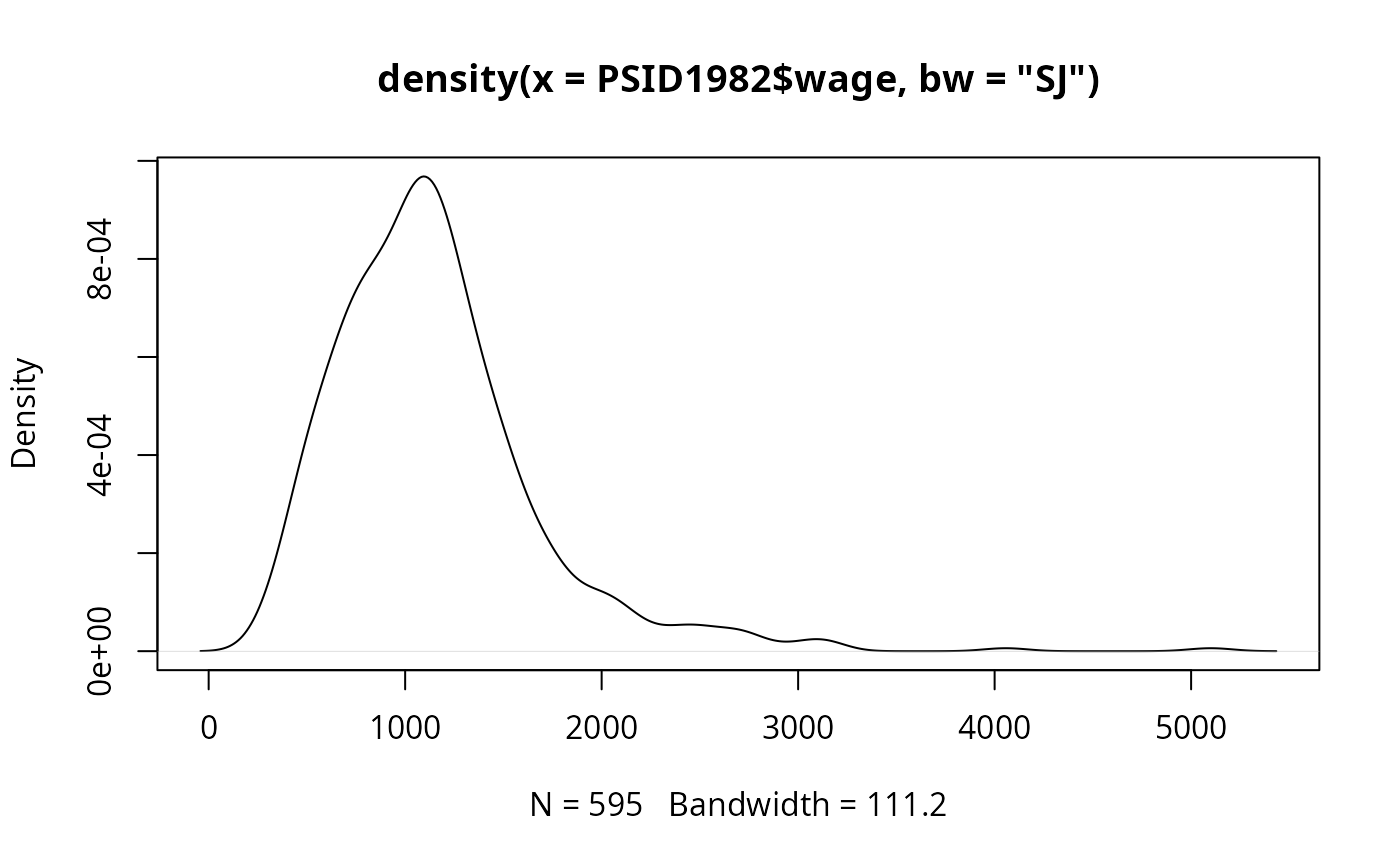
data("PSID1982")
plot(density(PSID1982$wage, bw = "SJ"))


## Baltagi (2002), Table 4.1
earn_lm <- lm(log(wage) ~ . + I(experience^2), data = PSID1982)
summary(earn_lm)
#> 
#> Call:
#> lm(formula = log(wage) ~ . + I(experience^2), data = PSID1982)
#> 
#> Residuals:
#>     Min      1Q  Median      3Q     Max 
#> -1.0271 -0.2292  0.0155  0.2231  1.1314 
#> 
#> Coefficients:
#>                   Estimate Std. Error t value Pr(>|t|)    
#> (Intercept)      5.5900930  0.1901125  29.404  < 2e-16 ***
#> experience       0.0293801  0.0065241   4.503 8.09e-06 ***
#> weeks            0.0034128  0.0026776   1.275 0.202973    
#> occupationblue  -0.1615216  0.0369073  -4.376 1.43e-05 ***
#> industryyes      0.0846626  0.0291637   2.903 0.003836 ** 
#> southyes        -0.0587635  0.0309069  -1.901 0.057755 .  
#> smsayes          0.1661912  0.0295510   5.624 2.90e-08 ***
#> marriedyes       0.0952370  0.0489277   1.946 0.052077 .  
#> genderfemale    -0.3245574  0.0607294  -5.344 1.30e-07 ***
#> unionyes         0.1062775  0.0316755   3.355 0.000845 ***
#> education        0.0571935  0.0065910   8.678  < 2e-16 ***
#> ethnicityafam   -0.1904220  0.0544118  -3.500 0.000502 ***
#> I(experience^2) -0.0004860  0.0001268  -3.833 0.000141 ***
#> ---
#> Signif. codes:  0 ‘***’ 0.001 ‘**’ 0.01 ‘*’ 0.05 ‘.’ 0.1 ‘ ’ 1
#> 
#> Residual standard error: 0.3256 on 582 degrees of freedom
#> Multiple R-squared:  0.4597,	Adjusted R-squared:  0.4485 
#> F-statistic: 41.26 on 12 and 582 DF,  p-value: < 2.2e-16
#> 

## Baltagi (2002), Table 13.1
union_lpm <- lm(I(as.numeric(union) - 1) ~ . - wage, data = PSID1982)
union_probit <- glm(union ~ . - wage, data = PSID1982, family = binomial(link = "probit"))
union_logit <- glm(union ~ . - wage, data = PSID1982, family = binomial)
## probit OK, logit and LPM rather different.