Benderly and Zwick Data: Inflation, Growth and Stock Returns

Time series data, 1952–1982.

Usage

data("BenderlyZwick")

Format

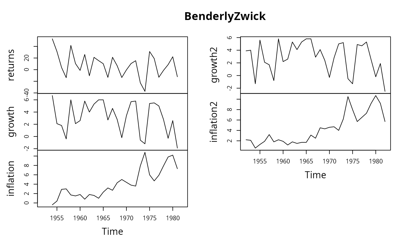
An annual multiple time series from 1952 to 1982 with 5 variables.

returns: real annual returns on stocks, measured using the Ibbotson-Sinquefeld data base.
growth: annual growth rate of output, measured by real GNP (from the given year to the next year).
inflation: inflation rate, measured as growth of price rate (from December of the previous year to December of the present year).
growth2: annual growth rate of real GNP as given by Baltagi.
inflation2: inflation rate as given by Baltagi

Source

The first three columns of the data are from Table 1 in Benderly and Zwick (1985). The remaining columns are taken from the online complements of Baltagi (2002). The first column is identical in both sources, the other two variables differ in their numeric values and additionally the growth series seems to be lagged differently. Baltagi (2002) states Lott and Ray (1992) as the source for his version of the data set.

References

Baltagi, B.H. (2002). Econometrics, 3rd ed. Berlin, Springer.

Benderly, J., and Zwick, B. (1985). Inflation, Real Balances, Output and Real Stock Returns. American Economic Review, 75, 1115–1123.

Lott, W.F., and Ray, S.C. (1992). Applied Econometrics: Problems with Data Sets. New York: The Dryden Press.

Zaman, A., Rousseeuw, P.J., and Orhan, M. (2001). Econometric Applications of High-Breakdown Robust Regression Techniques. Economics Letters, 71, 1–8.

Examples

data("BenderlyZwick")
plot(BenderlyZwick)


## Benderly and Zwick (1985), p. 1116
library("dynlm")
bz_ols <- dynlm(returns ~ growth + inflation,
  data = BenderlyZwick/100, start = 1956, end = 1981)
summary(bz_ols)
#> 
#> Time series regression with "ts" data:
#> Start = 1956, End = 1981
#> 
#> Call:
#> dynlm(formula = returns ~ growth + inflation, data = BenderlyZwick/100, 
#>     start = 1956, end = 1981)
#> 
#> Residuals:
#>       Min        1Q    Median        3Q       Max 
#> -0.279553 -0.073666 -0.004526  0.085589  0.224095 
#> 
#> Coefficients:
#>             Estimate Std. Error t value Pr(>|t|)    
#> (Intercept)  -0.1238     0.0833  -1.486 0.150747    
#> growth        5.2255     1.2702   4.114 0.000424 ***
#> inflation     0.1882     1.1053   0.170 0.866312    
#> ---
#> Signif. codes:  0 ‘***’ 0.001 ‘**’ 0.01 ‘*’ 0.05 ‘.’ 0.1 ‘ ’ 1
#> 
#> Residual standard error: 0.1333 on 23 degrees of freedom
#>   (0 observations deleted due to missingness)
#> Multiple R-squared:  0.5119,	Adjusted R-squared:  0.4695 
#> F-statistic: 12.06 on 2 and 23 DF,  p-value: 0.0002617
#> 

## Zaman, Rousseeuw and Orhan (2001)
## use larger period, without scaling
bz_ols2 <- dynlm(returns ~ growth + inflation,
  data = BenderlyZwick, start = 1954, end = 1981)
summary(bz_ols2)
#> 
#> Time series regression with "ts" data:
#> Start = 1954, End = 1981
#> 
#> Call:
#> dynlm(formula = returns ~ growth + inflation, data = BenderlyZwick, 
#>     start = 1954, end = 1981)
#> 
#> Residuals:
#>     Min      1Q  Median      3Q     Max 
#> -27.235  -8.478  -0.848   6.322  25.171 
#> 
#> Coefficients:
#>             Estimate Std. Error t value Pr(>|t|)   
#> (Intercept)   -3.586      8.581  -0.418   0.6796   
#> growth         4.778      1.368   3.492   0.0018 **
#> inflation     -1.046      1.145  -0.913   0.3698   
#> ---
#> Signif. codes:  0 ‘***’ 0.001 ‘**’ 0.01 ‘*’ 0.05 ‘.’ 0.1 ‘ ’ 1
#> 
#> Residual standard error: 15.02 on 25 degrees of freedom
#>   (2 observations deleted due to missingness)
#> Multiple R-squared:  0.4961,	Adjusted R-squared:  0.4558 
#> F-statistic: 12.31 on 2 and 25 DF,  p-value: 0.0001902
#>