Plot Survival Curves and Hazard Functions

Plot estimated survival curves, and for parametric survival models, plot hazard functions. There is an option to print the number of subjects at risk at the start of each time interval for certain models. Curves are automatically labeled at the points of maximum separation (using the labcurve function), and there are many other options for labeling that can be specified with the label.curves parameter. For example, different plotting symbols can be placed at constant x-increments and a legend linking the symbols with category labels can automatically positioned on the most empty portion of the plot.

If the fit is from psm and ggplot=TRUE is specified, a ggplot2 graphic will instead be produced using the survplot.orm function.

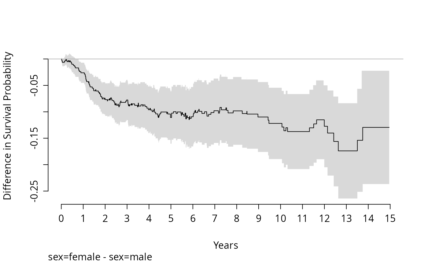
For the case of a two stratum analysis by npsurv, survdiffplot plots the difference in two Kaplan-Meier estimates along with approximate confidence bands for the differences, with a reference line at zero. The number of subjects at risk is optionally plotted. This number is taken as the minimum of the number of subjects at risk over the two strata. When conf='diffbands', survdiffplot instead does not make a new plot but adds a shaded polygon to an existing plot, showing the midpoint of two survival estimates plus or minus 1/2 the width of the confidence interval for the difference of two Kaplan-Meier estimates.

survplotp creates an interactive plotly graphic with shaded confidence bands for fits other than from orms. In the two strata case, it draws the 1/2 confidence bands for the difference in two probabilities centered at the midpoint of the probability estimates, so that where the two curves touch this band there is no significant difference (no multiplicity adjustment is made). For the two strata case, the two individual confidence bands have entries in the legend but are not displayed until the user clicks on the legend.

When code was from running npsurv on a multi-state/competing risk Surv object, survplot plots cumulative incidence curves properly accounting for competing risks. You must specify exactly one state/event cause to plot using the state argument. survplot will not plot multiple states on one graph. This can be accomplished using multiple calls with different values of state and specifying add=TRUE for all but the first call.

Usage

survplot(fit, ...)
survplotp(fit, ...)
# S3 method for class 'rms'
survplot(fit, ..., xlim,
         ylim=if(loglog) c(-5, 1.5) else if
                 (what == "survival" & missing(fun)) c(0, 1),
         xlab, ylab, time.inc,
         what=c("survival","hazard"),
         type=c("tsiatis","kaplan-meier"),
         conf.type=c("log","log-log","plain","none"),
         conf.int=FALSE, conf=c("bands","bars"), mylim=NULL,
         add=FALSE, label.curves=TRUE,
         abbrev.label=FALSE, levels.only=FALSE,
         lty, lwd=par("lwd"),
         col=1, col.fill=gray(seq(.95, .75, length=5)),
         adj.subtitle=TRUE, loglog=FALSE, fun,
         n.risk=FALSE, logt=FALSE, dots=FALSE, dotsize=.003,
         grid=NULL, srt.n.risk=0, sep.n.risk=0.056, adj.n.risk=1, 
         y.n.risk, cex.n.risk=.6, cex.xlab=par('cex.lab'),
         cex.ylab=cex.xlab, pr=FALSE, ggplot=FALSE)
# S3 method for class 'npsurv'
survplot(fit, xlim, 
         ylim, xlab, ylab, time.inc, state=NULL,
         conf=c("bands","bars","diffbands","none"), mylim=NULL,
         add=FALSE, label.curves=TRUE, abbrev.label=FALSE,
         levels.only=FALSE, lty,lwd=par('lwd'),
         col=1, col.fill=gray(seq(.95, .75, length=5)),
         loglog=FALSE, fun, n.risk=FALSE, aehaz=FALSE, times=NULL,
         logt=FALSE, dots=FALSE, dotsize=.003, grid=NULL,
         srt.n.risk=0, sep.n.risk=.056, adj.n.risk=1,
         y.n.risk, cex.n.risk=.6, cex.xlab=par('cex.lab'), cex.ylab=cex.xlab,
         pr=FALSE, ...)
# S3 method for class 'npsurv'
survplotp(fit, xlim, ylim, xlab, ylab, time.inc, state=NULL,
         conf=c("bands", "none"), mylim=NULL, abbrev.label=FALSE,
         col=colorspace::rainbow_hcl,  levels.only=TRUE,
         loglog=FALSE, fun=function(y) y, aehaz=FALSE, times=NULL,
         logt=FALSE, pr=FALSE, ...)
survdiffplot(fit, order=1:2, fun=function(y) y,
           xlim, ylim, xlab, ylab="Difference in Survival Probability",
           time.inc, conf.int, conf=c("shaded", "bands","diffbands","none"),
           add=FALSE, lty=1, lwd=par('lwd'), col=1,
           n.risk=FALSE, grid=NULL,
           srt.n.risk=0, adj.n.risk=1,
           y.n.risk, cex.n.risk=.6, cex.xlab=par('cex.lab'),
           cex.ylab=cex.xlab, convert=function(f) f)

Arguments

fit

result of fit (cph, psm, npsurv, survest.psm). For survdiffplot, fit must be the result of npsurv.

...

list of factors with names used in model. For fits from npsurv these arguments do not appear - all strata are plotted. Otherwise the first factor listed is the factor used to determine different survival curves. Any other factors are used to specify single constants to be adjusted to, when defaults given to fitting routine (through limits) are not used. The value given to factors is the original coding of data given to fit, except that for categorical or strata factors the text string levels may be specified. The form of values given to the first factor are none (omit the equal sign to use default range or list of all values if variable is discrete), "text" if factor is categorical, c(value1, value2, ...), or a function which returns a vector, such as seq(low,high,by=increment). Only the first factor may have the values omitted. In this case the Low effect, Adjust to, and High effect values will be used from datadist if the variable is continuous. For variables not defined to datadist, you must specify non-missing constant settings (or a vector of settings for the one displayed variable). Note that since npsurv objects do not use the variable list in ..., you can specify any extra arguments to labcurve by adding them at the end of the list of arguments. For survplotp ... (e.g., height, width) is passed to plotly::plot_ly.

xlim

a vector of two numbers specifiying the x-axis range for follow-up time. Default is (0,maxtime) where maxtime was the pretty()d version of the maximum follow-up time in any stratum, stored in fit$maxtime. If logt=TRUE, default is (1, log(maxtime)).

ylim

y-axis limits. Default is c(0,1) for survival, and c(-5,1.5) if loglog=TRUE. If fun or loglog=TRUE are given and ylim is not, the limits will be computed from the data. For what="hazard", default limits are computed from the first hazard function plotted.

xlab

x-axis label. Default is units attribute of failure time variable given to Surv.

ylab

y-axis label. Default is "Survival Probability" or "log(-log Survival Probability)". If fun is given, the default is "". For what="hazard", the default is "Hazard Function". For a multi-state/competing risk application the default is "Cumulative Incidence".

time.inc

time increment for labeling the x-axis and printing numbers at risk. If not specified, the value of time.inc stored with the model fit will be used.

state

the state/event cause to use in plotting if the fit was for a multi-state/competing risk Surv object

type

specifies type of estimates, "tsiatis" (the default) or "kaplan-meier". "tsiatis" here corresponds to the Breslow estimator. This is ignored if survival estimates stored with surv=TRUE are being used. For fits from npsurv, this argument is also ignored, since it is specified as an argument to npsurv.

conf.type

specifies the basis for confidence limits. This argument is ignored for fits from npsurv.

conf.int

Default is FALSE. Specify e.g. .95 to plot 0.95 confidence bands. For fits from parametric survival models, or Cox models with x=TRUE and y=TRUE specified to the fit, the exact asymptotic formulas will be used to compute standard errors, and confidence limits are based on log(-log S(t)) if loglog=TRUE. If x=TRUE and y=TRUE were not specified to cph but surv=TRUE was, the standard errors stored for the underlying survival curve(s) will be used. These agree with the former if predictions are requested at the mean value of X beta or if there are only stratification factors in the model. This argument is ignored for fits from npsurv, which must have previously specified confidence interval specifications. For survdiffplot if conf.int is not specified, the level used in the call to npsurv will be used.

conf

"bars" for confidence bars at each time.inc time point. If the fit was from cph(..., surv=TRUE), the time.inc used will be that stored with the fit. Use conf="bands" (the default) for bands using standard errors at each failure time. For npsurv objects only, conf may also be "none", indicating that confidence interval information stored with the npsurv result should be ignored. For npsurv and survdiffplot, conf may be "diffbands" whereby a shaded region is drawn for comparing two curves. The polygon is centered at the midpoint of the two survival estimates and the height of the polygon is 1/2 the width of the approximate conf.int pointwise confidence region. Survival curves not overlapping the shaded area are approximately significantly different at the 1 - conf.int level.

mylim

used to curtail computed ylim. When ylim is not given by the user, the computed limits are expanded to force inclusion of the values specified in mylim.

what

defaults to "survival" to plot survival estimates. Set to "hazard" or an abbreviation to plot the hazard function (for psm fits only). Confidence intervals are not available for what="hazard".

add

set to TRUE to add curves to an existing plot.

label.curves

default is TRUE to use labcurve to label curves where they are farthest apart. Set label.curves to a list to specify options to labcurve, e.g., label.curves=list(method="arrow", cex=.8). These option names may be abbreviated in the usual way arguments are abbreviated. Use for example label.curves=list(keys=1:5) to draw symbols (as in pch=1:5 - see points) on the curves and automatically position a legend in the most empty part of the plot. Set label.curves=FALSE to suppress drawing curve labels. The col, lty, lwd, and type parameters are automatically passed to labcurve, although you can override them here. To distinguish curves by line types and still have labcurve construct a legend, use for example label.curves=list(keys="lines"). The negative value for the plotting symbol will suppress a plotting symbol from being drawn either on the curves or in the legend.

abbrev.label

set to TRUE to abbreviate() curve labels that are plotted

levels.only

set to TRUE to remove variablename= from the start of curve labels.

lty

vector of line types to use for different factor levels. Default is c(1,3,4,5,6,7,...).

lwd

vector of line widths to use for different factor levels. Default is current par setting for lwd.

col

color for curve, default is 1. Specify a vector to assign different colors to different curves. For survplotp, col is a vector of colors corresponding to strata, or a function that will be called to generate such colors.

col.fill

a vector of colors to used in filling confidence bands

adj.subtitle

set to FALSE to suppress plotting subtitle with levels of adjustment factors not plotted. Defaults to TRUE. This argument is ignored for npsurv.

loglog

set to TRUE to plot log(-log Survival) instead of Survival

fun

specifies any function to translate estimates and confidence limits before plotting. If the fit is a multi-state object the default for fun is function(y) 1 - y to draw cumulative incidence curves.

logt

set to TRUE to plot log(t) instead of t on the x-axis

n.risk

set to TRUE to add number of subjects at risk for each curve, using the surv.summary created by cph or using the failure times used in fitting the model if y=TRUE was specified to the fit or if the fit was from npsurv. The numbers are placed at the bottom of the graph unless y.n.risk is given. If the fit is from survest.psm, n.risk does not apply.

srt.n.risk

angle of rotation for leftmost number of subjects at risk (since this number may run into the second or into the y-axis). Default is 0.

adj.n.risk

justification for leftmost number at risk. Default is 1 for right justification. Use 0 for left justification, .5 for centered.

sep.n.risk

multiple of upper y limit - lower y limit for separating lines of text containing number of subjects at risk. Default is .056*(ylim[2]-ylim[1]).

y.n.risk

When n.risk=TRUE, the default is to place numbers of patients at risk above the x-axis. You can specify a y-coordinate for the bottom line of the numbers using y.n.risk. Specify y.n.risk='auto' to place the numbers below the x-axis at a distance of 1/3 of the range of ylim.

cex.n.risk

character size for number of subjects at risk (when n.risk is TRUE)

cex.xlab

cex for x-axis label

cex.ylab

cex for y-axis label

dots

set to TRUE to plot a grid of dots. Will be plotted at every time.inc (see cph) and at survival increments of .1 (if d>.4), .05 (if .2 < d <= .4), or .025 (if d <= .2), where d is the range of survival displayed.

dotsize

size of dots in inches

grid

defaults to NULL (not drawing grid lines). Set to TRUE to plot gray(.8) grid lines, or specify any color.

pr

set to TRUE to print survival curve coordinates used in the plots

ggplot

set to TRUE to use survplot.orm to draw the curves instead, for a psm fit

aehaz

set to TRUE to add number of events and exponential distribution hazard rate estimates in curve labels. For competing risk data the number of events is for the cause of interest, and the hazard rate is the number of events divided by the sum of all failure and censoring times.

times

a numeric vector of times at which to compute cumulative incidence probability estimates to add to curve labels

order

an integer vector of length two specifying the order of groups when computing survival differences. The default of 1:2 indicates that the second group is subtracted from the first. Specify order=2:1 to instead subtract the first from the second. A subtitle indicates what was done.

convert

a function to convert the output of summary.survfitms to pick off the data needed for a single state

Value

list with components adjust (text string specifying adjustment levels) and curve.labels (vector of text strings corresponding to levels of factor used to distinguish curves). For npsurv, the returned value is the vector of strata labels, or NULL if there are no strata.

Side Effects

plots. If par()$mar[4] < 4, issues par(mar=) to increment mar[4] by 2 if n.risk=TRUE and add=FALSE. The user may want to reset par(mar) in this case to not leave such a wide right margin for plots. You usually would issue par(mar=c(5,4,4,2)+.1).

Details

survplot will not work for Cox models with time-dependent covariables. Use survest or survfit for that purpose.

There is a set a system option mgp.axis.labels to allow x and y-axes to have differing mgp graphical parameters (see par). This is important when labels for y-axis tick marks are to be written horizontally (par(las=1)), as a larger gap between the labels and the tick marks are needed. You can set the axis-specific 2nd component of mgp using mgp.axis.labels(c(xvalue,yvalue)).

References

Boers M (2004): Null bar and null zone are better than the error bar to compare group means in graphs. J Clin Epi 57:712-715.

See also

datadist, rms, cph, psm, survest, predictrms, plot.Predict, ggplot.Predict, units, errbar, survfit, survreg.distributions, labcurve, mgp.axis, par,

Examples

# Simulate data from a population model in which the log hazard
# function is linear in age and there is no age x sex interaction
require(survival)
n <- 1000
set.seed(731)
age <- 50 + 12*rnorm(n)
label(age) <- "Age"
sex <- factor(sample(c('male','female'), n, TRUE))
cens <- 15*runif(n)
h <- .02*exp(.04*(age-50)+.8*(sex=='female'))
dt <- -log(runif(n))/h
label(dt) <- 'Follow-up Time'
e <- ifelse(dt <= cens,1,0)
dt <- pmin(dt, cens)
units(dt) <- "Year"
dd <- datadist(age, sex)
options(datadist='dd')
S <- Surv(dt,e)

# When age is in the model by itself and we predict at the mean age,
# approximate confidence intervals are ok

f <- cph(S ~ age, surv=TRUE)
#> Error in Design(data, formula, specials = c("strat", "strata")): dataset dd not found for options(datadist=)
survplot(f, age=mean(age), conf.int=.95)
#> Error: object 'f' not found
g <- cph(S ~ age, x=TRUE, y=TRUE)
#> Error in Design(data, formula, specials = c("strat", "strata")): dataset dd not found for options(datadist=)
survplot(g, age=mean(age), conf.int=.95, add=TRUE, col='red', conf='bars')
#> Error: object 'g' not found

# Repeat for an age far from the mean; not ok
survplot(f, age=75, conf.int=.95)
#> Error: object 'f' not found
survplot(g, age=75, conf.int=.95, add=TRUE, col='red', conf='bars')
#> Error: object 'g' not found


#Plot stratified survival curves by sex, adj for quadratic age effect
# with age x sex interaction (2 d.f. interaction)

f <- cph(S ~ pol(age,2)*strat(sex), x=TRUE, y=TRUE)
#> Error in Design(data, formula, specials = c("strat", "strata")): dataset dd not found for options(datadist=)
#or f <- psm(S ~ pol(age,2)*sex)
Predict(f, sex, age=c(30,50,70))
#> Error: object 'f' not found
survplot(f, sex, n.risk=TRUE, levels.only=TRUE)   #Adjust age to median
#> Error: object 'f' not found
survplot(f, sex, logt=TRUE, loglog=TRUE)   #Check for Weibull-ness (linearity)
#> Error: object 'f' not found
survplot(f, sex=c("male","female"), age=50)
#> Error: object 'f' not found
                                        #Would have worked without datadist
                                        #or with an incomplete datadist
survplot(f, sex, label.curves=list(keys=c(2,0), point.inc=2))
#> Error: object 'f' not found
                                        #Identify curves with symbols


survplot(f, sex, label.curves=list(keys=c('m','f')))
#> Error: object 'f' not found
                                        #Identify curves with single letters


#Plots by quintiles of age, adjusting sex to male
options(digits=3)
survplot(f, age=quantile(age,(1:4)/5), sex="male")
#> Error: object 'f' not found


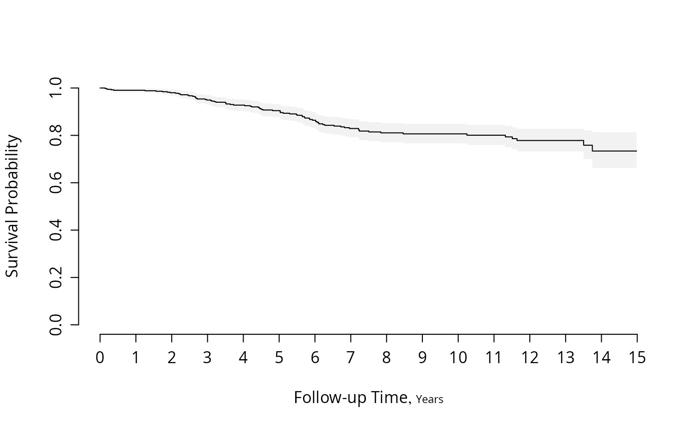
#Plot survival Kaplan-Meier survival estimates for males
f <- npsurv(S ~ 1, subset=sex=="male")
survplot(f)



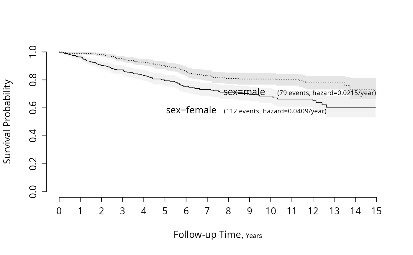
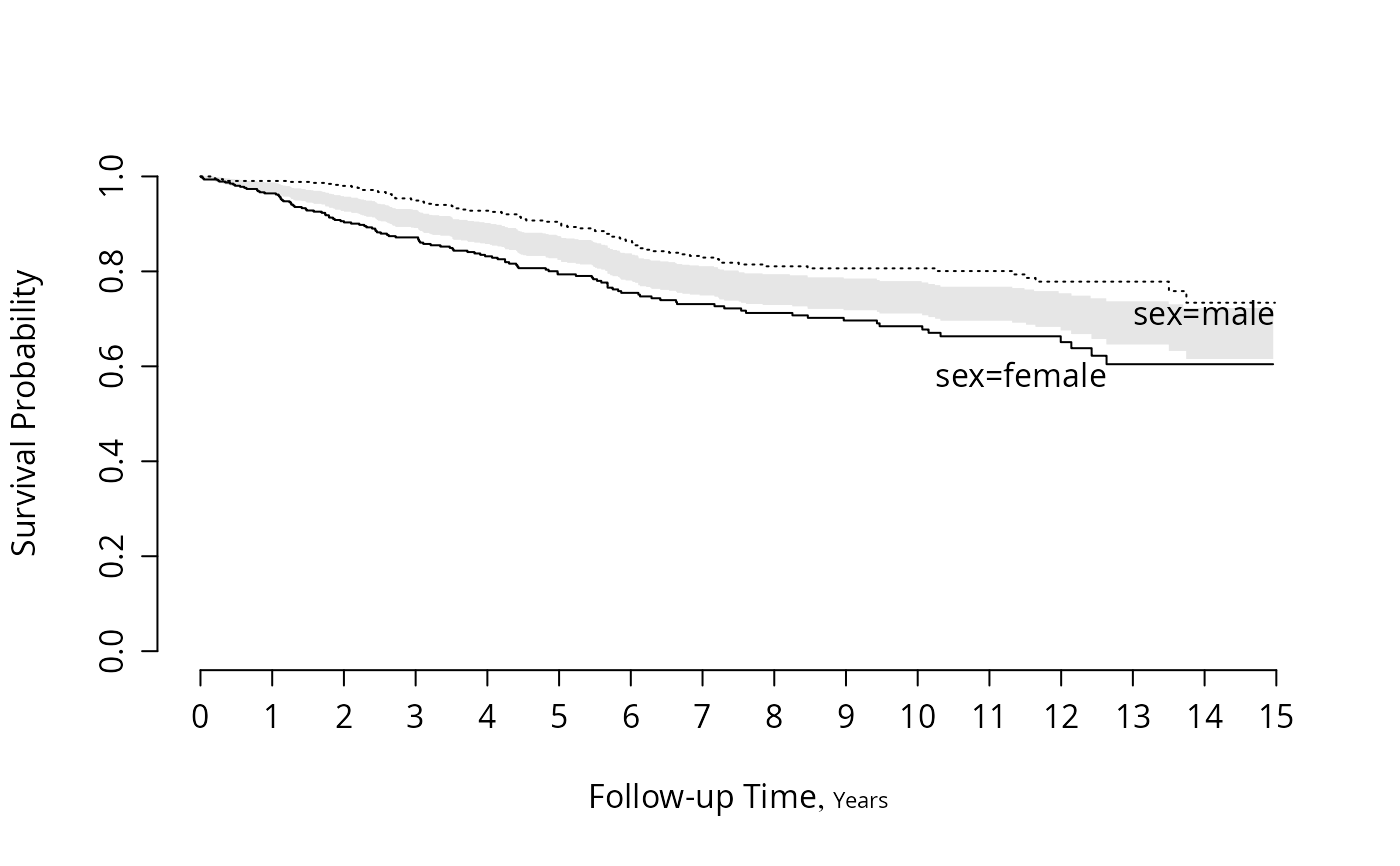
#Plot survival for both sexes and show exponential hazard estimates
f <- npsurv(S ~ sex)
survplot(f, aehaz=TRUE)

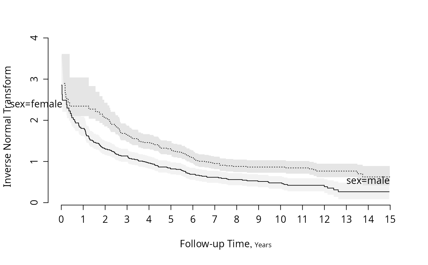
#Check for log-normal and log-logistic fits
survplot(f, fun=qnorm, ylab="Inverse Normal Transform")

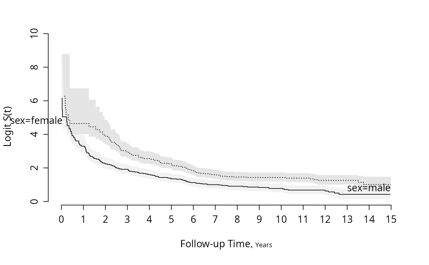
survplot(f, fun=function(y)log(y/(1-y)), ylab="Logit S(t)")


#Plot the difference between sexes
survdiffplot(f)


#Similar but show half-width of confidence intervals centered
#at average of two survival estimates
#See Boers (2004)
survplot(f, conf='diffbands')


options(datadist=NULL)
if (FALSE) { # \dontrun{
#
# Time to progression/death for patients with monoclonal gammopathy
# Competing risk curves (cumulative incidence)
# status variable must be a factor with first level denoting right censoring
m <- upData(mgus1, stop = stop / 365.25, units=c(stop='years'),
            labels=c(stop='Follow-up Time'), subset=start == 0)
f <- npsurv(Surv(stop, event) ~ 1, data=m)

# Use survplot for enhanced displays of cumulative incidence curves for
# competing risks

survplot(f, state='pcm', n.risk=TRUE, xlim=c(0, 20), ylim=c(0, .5), col=2)
survplot(f, state='death', aehaz=TRUE, col=3,
         label.curves=list(keys='lines'))
f <- npsurv(Surv(stop, event) ~ sex, data=m)
survplot(f, state='death', aehaz=TRUE, n.risk=TRUE, conf='diffbands',
         label.curves=list(keys='lines'))

# Plot survival curves estimated from an ordinal semiparametric model
f <- orm(Ocens(y, ifelse(y <= cens, y, Inf)) ~ age)
survplot(f, age=c(30, 50))
} # }