Time series plotting methods
xyplot.ts.RdThis function handles time series plotting, including cut-and-stack plots. Examples are given of superposing, juxtaposing and styling different time series.
Usage
# S3 method for class 'ts'
xyplot(x, data = NULL,
       screens = if (superpose) 1 else colnames(x),
       ...,
       superpose = FALSE,
       cut = FALSE,
       type = "l",
       col = NULL,
       lty = NULL,
       lwd = NULL,
       pch = NULL,
       cex = NULL,
       fill = NULL,
       auto.key = superpose,
       panel = if (superpose) "panel.superpose"
               else "panel.superpose.plain",
       par.settings = list(),
       layout = NULL, as.table = TRUE,
       xlab = "Time", ylab = NULL,
       default.scales = list(y = list(relation =
           if (missing(cut)) "free" else "same")))
Arguments
- x
an object of class
ts, which may be multi-variate, i.e. have a matrix structure with multiple columns.- data
not used, and must be left as
NULL.- ...
additional arguments passed to
xyplot, which may pass them on topanel.xyplot.- screens
factor (or coerced to factor) whose levels specify which panel each series is to be plotted in.
screens = c(1, 2, 1)would plot series 1, 2 and 3 in panels 1, 2 and 1. May also be a named list, see Details below.- superpose
overlays all series in one panel (via
screens = 1) and uses grouped style settings (fromtrellis.par.get("superpose.line"), etc). Note that this is just a convenience argument: its only action is to change the default values of other arguments.- cut
defines a cut-and-stack plot.
cutcan be alistof arguments to the functionequal.count, i.e.number(number of intervals to divide into) andoverlap(the fraction of overlap between cuts, default 0.5). Ifcutis numeric this is passed as thenumberargument.cut = TRUEtries to choose an appropriate number of cuts (up to a maximum of 6), usingbanking, and assuming a square plot region. This should have the effect of minimising wasted space whenaspect = "xy".- type, col, lty, lwd, pch, cex, fill
graphical arguments, which are processed and eventually passed to
panel.xyplot. These arguments can also be vectors or (named) lists, see Details for more information.- auto.key
a logical, or a list describing how to draw a key. See the
auto.keyentry inxyplot. The default here is to draw lines, not points, and any specified style arguments should show up automatically.- panel
the panel function. It is recommended to leave this alone, but one can pass a
panel.groupsargument which is handled bypanel.superposefor each series.- par.settings
style settings beyond the standard
col,lty,lwd, etc; seetrellis.par.setandsimpleTheme.- layout
numeric vector of length 2 specifying number of columns and rows in the plot. The default is to fill columns with up to 6 rows.
- as.table
to draw panels from top to bottom. The order is determined by the order of columns in
x.- xlab, ylab
X axis and Y axis labels; see
xyplot. Note in particular thatylabmay be a character vector, in which case the labels are spaced out equally, to correspond to the panels; but NOTE in this case the vector should be reversed OR the argumentas.tableset toFALSE.- default.scales
scalesspecification. The default is set to have"free"Y axis scales unlesscutis given. Note, users should pass thescalesargument rather thandefault.scales.
Details
The handling of several graphical parameters is more
flexible for multivariate series. These parameters can be
vectors of the same length as the number of series plotted or
are recycled if shorter. They can also be (partially) named list, e.g.,
list(A = c(1,2), c(3,4)) in which c(3, 4) is the
default value and c(1, 2) the value only for series A.
The screens argument can be specified in a similar way.
Some examples are given below.
Value
An object of class "trellis". The
update method can be used to
update components of the object and the
print method (usually called by
default) will plot it on an appropriate plotting device.
Author
Gabor Grothendieck, Achim Zeileis, Deepayan Sarkar and Felix Andrews felix@nfrac.org.
The first two authors developed xyplot.ts in their zoo
package, including the screens approach. The third author
developed a different xyplot.ts for cut-and-stack plots in the
latticeExtra package. The final author fused these together.
References
Sarkar, Deepayan (2008) Lattice: Multivariate Data Visualization with R, Springer. http://lmdvr.r-forge.r-project.org/ (cut-and-stack plots)
See also
xyplot,
panel.xyplot,
plot.ts,
ts,
xyplot.zoo in the zoo package.
Examples
xyplot(ts(c(1:10,10:1)))
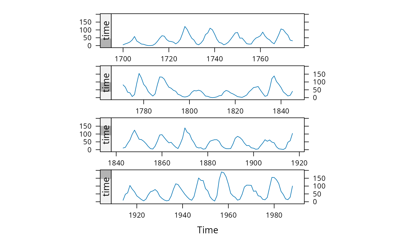
 ### Figure 14.1 from Sarkar (2008)
xyplot(sunspot.year, aspect = "xy",
strip = FALSE, strip.left = TRUE,
cut = list(number = 4, overlap = 0.05))
### Figure 14.1 from Sarkar (2008)
xyplot(sunspot.year, aspect = "xy",
strip = FALSE, strip.left = TRUE,
cut = list(number = 4, overlap = 0.05))
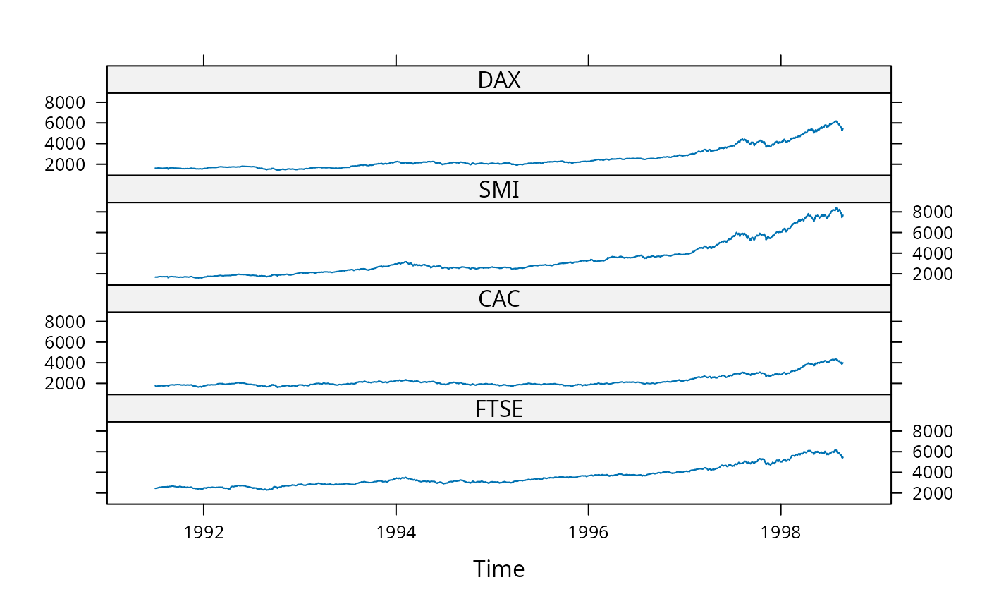
 ### A multivariate example; first juxtaposed, then superposed
xyplot(EuStockMarkets, scales = list(y = "same"))
### A multivariate example; first juxtaposed, then superposed
xyplot(EuStockMarkets, scales = list(y = "same"))
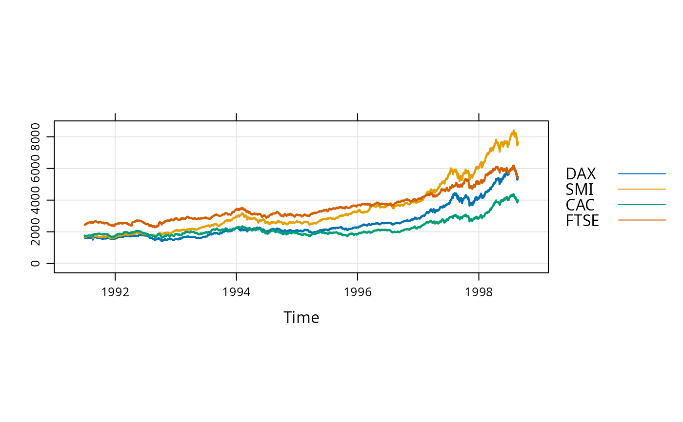
 xyplot(EuStockMarkets, superpose = TRUE, aspect = "xy", lwd = 2,
type = c("l","g"), ylim = c(0, max(EuStockMarkets)))
xyplot(EuStockMarkets, superpose = TRUE, aspect = "xy", lwd = 2,
type = c("l","g"), ylim = c(0, max(EuStockMarkets)))
 ### Examples using screens (these two are identical)
xyplot(EuStockMarkets, screens = c(rep("Continental", 3), "UK"))
### Examples using screens (these two are identical)
xyplot(EuStockMarkets, screens = c(rep("Continental", 3), "UK"))
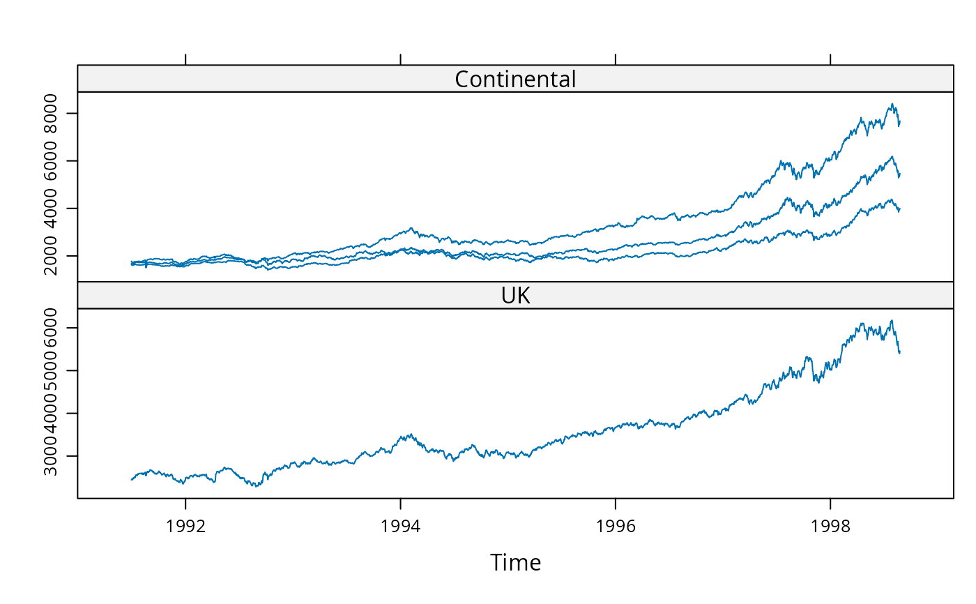 xyplot(EuStockMarkets, screens = list(FTSE = "UK", "Continental"))
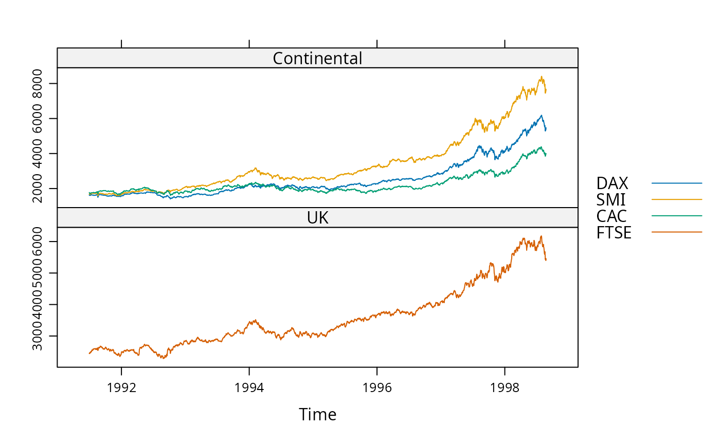
 ### Automatic group styles
xyplot(EuStockMarkets, screens = list(FTSE = "UK", "Continental"),
superpose = TRUE)
### Automatic group styles
xyplot(EuStockMarkets, screens = list(FTSE = "UK", "Continental"),
superpose = TRUE)
 xyplot(EuStockMarkets, screens = list(FTSE = "UK", "Continental"),
superpose = TRUE, xlim = extendrange(1996:1998),
par.settings = standard.theme(color = FALSE))
xyplot(EuStockMarkets, screens = list(FTSE = "UK", "Continental"),
superpose = TRUE, xlim = extendrange(1996:1998),
par.settings = standard.theme(color = FALSE))
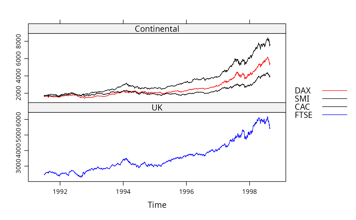
 ### Specifying styles for series by name
xyplot(EuStockMarkets, screens = list(FTSE = "UK", "Continental"),
col = list(DAX = "red", FTSE = "blue", "black"), auto.key = TRUE)
### Specifying styles for series by name
xyplot(EuStockMarkets, screens = list(FTSE = "UK", "Continental"),
col = list(DAX = "red", FTSE = "blue", "black"), auto.key = TRUE)
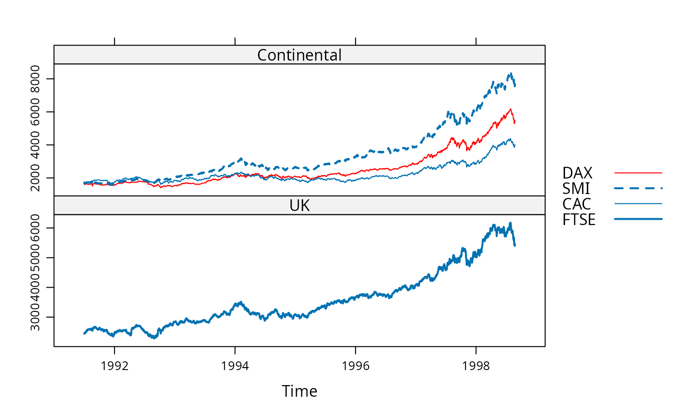
 xyplot(EuStockMarkets, screens = list(FTSE = "UK", "Continental"),
col = list(DAX = "red"), lty = list(SMI = 2), lwd = 1:2,
auto.key = TRUE)
xyplot(EuStockMarkets, screens = list(FTSE = "UK", "Continental"),
col = list(DAX = "red"), lty = list(SMI = 2), lwd = 1:2,
auto.key = TRUE)
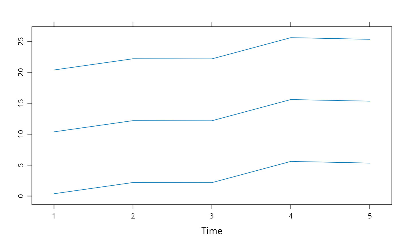
 ### Example with simpler data, few data points
set.seed(1)
z <- ts(cbind(a = 1:5, b = 11:15, c = 21:25) + rnorm(5))
xyplot(z, screens = 1)
### Example with simpler data, few data points
set.seed(1)
z <- ts(cbind(a = 1:5, b = 11:15, c = 21:25) + rnorm(5))
xyplot(z, screens = 1)
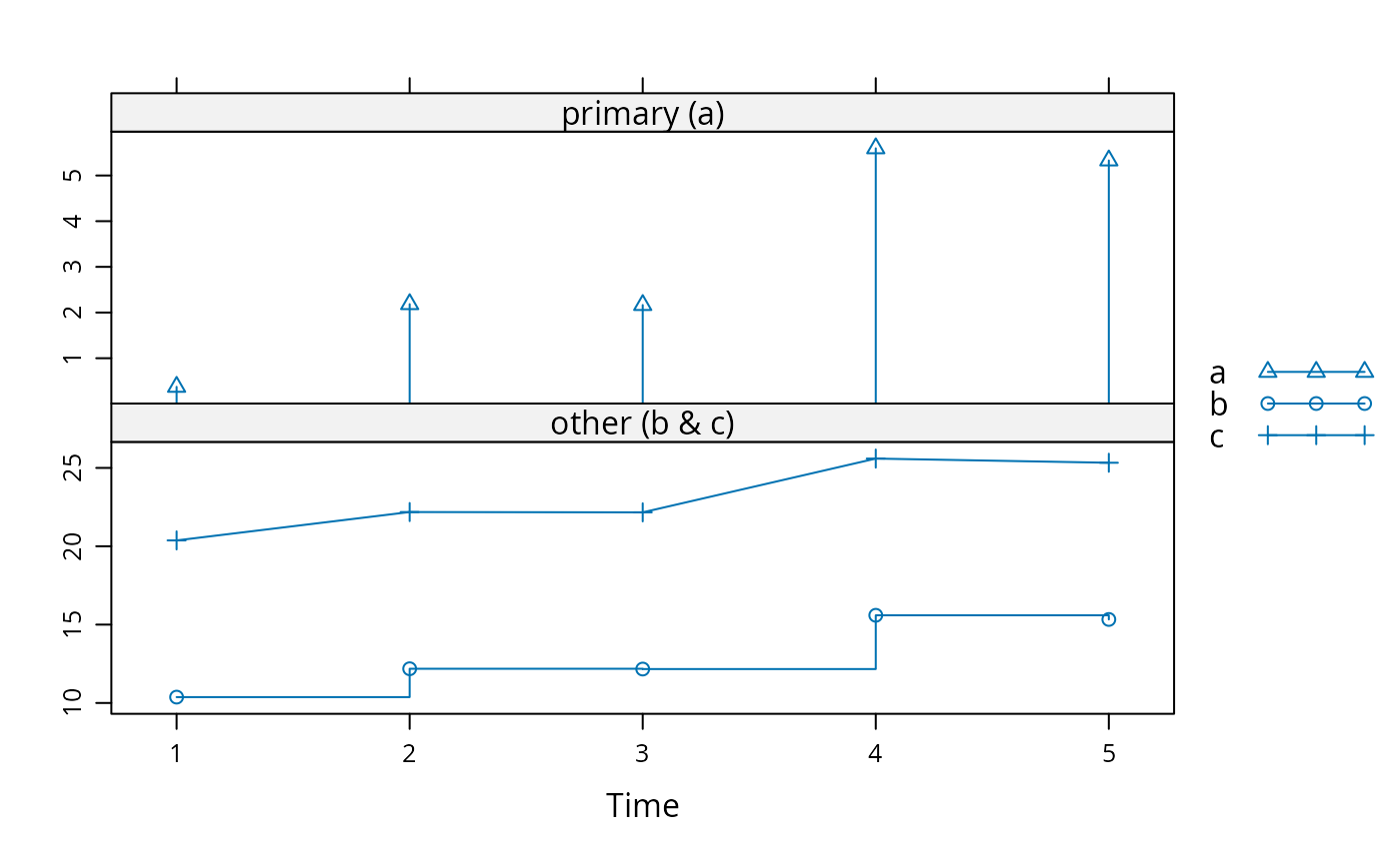
 xyplot(z, screens = list(a = "primary (a)", "other (b & c)"),
type = list(a = c("p", "h"), b = c("p", "s"), "o"),
pch = list(a = 2, c = 3), auto.key = list(type = "o"))
xyplot(z, screens = list(a = "primary (a)", "other (b & c)"),
type = list(a = c("p", "h"), b = c("p", "s"), "o"),
pch = list(a = 2, c = 3), auto.key = list(type = "o"))