Level plots and contour plots — B.06 levelplot • lattice

Draws false color level plots and contour plots.

Usage

levelplot(x, data, ...)
contourplot(x, data, ...)

# S3 method for class 'formula'
levelplot(x,
          data,
          allow.multiple = is.null(groups) || outer,
          outer = TRUE,
          aspect = "fill",
          panel = if (useRaster) lattice.getOption("panel.levelplot.raster")
                  else lattice.getOption("panel.levelplot"),
          prepanel = NULL,
          scales = list(),
          strip = TRUE,
          groups = NULL,
          xlab,
          xlim,
          ylab,
          ylim,
          at,
          cuts = 15,
          pretty = FALSE,
          region = TRUE,
          drop.unused.levels =
              lattice.getOption("drop.unused.levels"),
          ...,
          useRaster = FALSE,
          lattice.options = NULL,
          default.scales = list(),
          default.prepanel =
              lattice.getOption("prepanel.default.levelplot"),
          colorkey = region,
          col.regions,
          alpha.regions,
          subset = TRUE)

# S3 method for class 'formula'
contourplot(x,
            data,
            panel = lattice.getOption("panel.contourplot"),
            default.prepanel =
                lattice.getOption("prepanel.default.contourplot"),
            cuts = 7,
            labels = TRUE,
            contour = TRUE,
            pretty = TRUE,
            region = FALSE,
            ...)

# S3 method for class 'data.frame'
levelplot(x, data = NULL, formula = data, ...)

# S3 method for class 'data.frame'
contourplot(x, data = NULL, formula = data, ...)

# S3 method for class 'table'
levelplot(x, data = NULL, aspect = "iso", ..., xlim, ylim)

# S3 method for class 'table'
contourplot(x, data = NULL, aspect = "iso", ..., xlim, ylim)

# S3 method for class 'matrix'
levelplot(x, data = NULL, aspect = "iso",
          ..., xlim, ylim,
          row.values = seq_len(nrow(x)),
          column.values = seq_len(ncol(x)))

# S3 method for class 'matrix'
contourplot(x, data = NULL, aspect = "iso",
            ..., xlim, ylim,
            row.values = seq_len(nrow(x)),
            column.values = seq_len(ncol(x)))


# S3 method for class 'array'
levelplot(x, data = NULL, ...)

# S3 method for class 'array'
contourplot(x, data = NULL, ...)

Arguments

x

for the formula method, a formula of the form z ~ x * y | g1 * g2 * ..., where z is a numeric response, and x, y are numeric values evaluated on a rectangular grid. g1, g2, ... are optional conditional variables, and must be either factors or shingles if present.

Calculations are based on the assumption that all x and y values are evaluated on a grid (defined by their unique values). The function will not return an error if this is not true, but the display might not be meaningful. However, the x and y values need not be equally spaced.

Both levelplot and wireframe have methods for matrix, array, and table objects, in which case x provides the z vector described above, while its rows and columns are interpreted as the x and y vectors respectively. This is similar to the form used in filled.contour and image. For higher-dimensional arrays and tables, further dimensions are used as conditioning variables. Note that the dimnames may be duplicated; this is handled by calling make.unique to make the names unique (although the original labels are used for the x- and y-axes).

data

For the formula methods, an optional data frame in which variables in the formula (as well as groups and subset, if any) are to be evaluated. Usually ignored with a warning in other cases.

formula

The formula to be used for the "data.frame" methods. See documentation for argument x for details.

row.values, column.values

Optional vectors of values that define the grid when x is a matrix. row.values and column.values must have the same lengths as nrow(x) and ncol(x) respectively. By default, row and column numbers.

panel

panel function used to create the display, as described in xyplot

aspect

For the matrix methods, the default aspect ratio is chosen to make each cell square. The usual default is aspect="fill", as described in xyplot.

at

A numeric vector giving breakpoints along the range of z. Contours (if any) will be drawn at these heights, and the regions in between would be colored using col.regions. In the latter case, values outside the range of at will not be drawn at all. This serves as a way to limit the range of the data shown, similar to what a zlim argument might have been used for. However, this also means that when supplying at explicitly, one has to be careful to include values outside the range of z to ensure that all the data are shown.

at can have length one only if region=FALSE.

col.regions

color vector to be used if regions is TRUE. The general idea is that this should be a color vector of moderately large length (longer than the number of regions. By default this is 100). It is expected that this vector would be gradually varying in color (so that nearby colors would be similar). When the colors are actually chosen, they are chosen to be equally spaced along this vector. When there are more regions than colors in col.regions, the colors are recycled. The actual color assignment is performed by level.colors, which is documented separately.

alpha.regions

Numeric, specifying alpha transparency (works only on some devices)

colorkey

A logical flag specifying whether a colorkey is to be drawn alongside the plot, or a list describing the colorkey. The list may contain the following components:

space:

location of the colorkey, can be one of "left", "right", "top" and "bottom". Defaults to "right".

x, y:

location, currently unused

col:

A color ramp specification, as in the col.regions argument in level.colors

at:

A numeric vector specifying where the colors change. must be of length 1 more than the col vector.

tri.lower, tri.upper:

Logical or numeric controlling whether the first and last intervals should be triangular instead of rectangular. With the default value (NA), this happens only if the corresponding extreme at values are -Inf or Inf respectively, and the triangles occupy 5% of the total length of the color key. If numeric and between 0 and 0.25, these give the corresponding fraction, which is again 5% when specified as TRUE.

labels:

A character vector for labelling the at values, or more commonly, a list describing characteristics of the labels. This list may include components labels, at, cex, col, rot, font, fontface and fontfamily.

title:

Usually a character vector or expression providing a title for the colorkey, or a list controlling the title in further detail, or an arbitrary "grob". For details of how the list form is interpreted, see the entry for main in xyplot; generally speaking, the actual label should be specified as the label component (which may be unnamed if it is the first component), and the remaining arguments are used as appropriate in a call to textGrob.

Further control of the placement of the title is possible through the component title.control. In particular, if a rot component is not specified, its default depends on the value of title.control$side (0 for top or bottom, and 90 for left or right).

title defaults to NULL, which means no title is drawn.

title.control:

A list providing control over the placement of a title, if specified. Currently two components are honoured: side can take values "top", "bottom", "left", and "right", and specifies the side of the colorkey on which the title is to be placed. Defaults to the value of the "space" component. padding is a multiplier for the default amount of padding between the title and the colorkey.

tick.number:

The approximate number of ticks desired.

tck:

A (scalar) multipler for tick lengths.

corner:

Interacts with x, y; currently unimplemented

width:

The width of the key

height:

The length of key as a fraction of the appropriate side of plot.

raster:

A logical flag indicating whether the colorkey should be rendered as a raster image using grid.raster. See also panel.levelplot.raster.

interpolate:

Logical flag, passed to rasterGrob when raster=TRUE.

axis.line:

A list giving graphical parameters for the color key boundary and tick marks. Defaults to trellis.par.get("axis.line").

axis.text:

A list giving graphical parameters for the tick mark labels on the color key. Defaults to trellis.par.get("axis.text").

contour

A logical flag, indicating whether to draw contour lines.

cuts

The number of levels the range of z would be divided into.

labels

Typically a logical indicating whether contour lines should be labelled, but other possibilities for more sophisticated control exists. Details are documented in the help page for panel.levelplot, to which this argument is passed on unchanged. That help page also documents the label.style argument, which affects how the labels are rendered.

pretty

A logical flag, indicating whether to use pretty cut locations and labels.

region

A logical flag, indicating whether regions between contour lines should be filled as in a level plot.

allow.multiple, outer, prepanel, scales, strip, groups, xlab, xlim, ylab, ylim, drop.unused.levels, lattice.options, default.scales, subset

These arguments are described in the help page for xyplot.

default.prepanel

Fallback prepanel function. See xyplot.

...

Further arguments may be supplied. Some are processed by levelplot or contourplot, and those that are unrecognized are passed on to the panel function.

useRaster

A logical flag indicating whether raster representations should be used, both for the false color image and the color key (if present). Effectively, setting this to TRUE changes the default panel function from panel.levelplot to panel.levelplot.raster, and sets the default value of colorkey$raster to TRUE.

Note that panel.levelplot.raster provides only a subset of the features of panel.levelplot, but setting useRaster=TRUE will not check whether any of the additional features have been requested.

Not all devices support raster images. For devices that appear to lack support, useRaster=TRUE will be ignored with a warning.

Details

These and all other high level Trellis functions have several arguments in common. These are extensively documented only in the help page for xyplot, which should be consulted to learn more detailed usage.

Other useful arguments are mentioned in the help page for the default panel function panel.levelplot (these are formally arguments to the panel function, but can be specified in the high level calls directly).

References

Sarkar, Deepayan (2008) Lattice: Multivariate Data Visualization with R, Springer. http://lmdvr.r-forge.r-project.org/

Value

An object of class "trellis". The update method can be used to update components of the object and the print method (usually called by default) will plot it on an appropriate plotting device.

Author

Deepayan Sarkar Deepayan.Sarkar@R-project.org

Examples

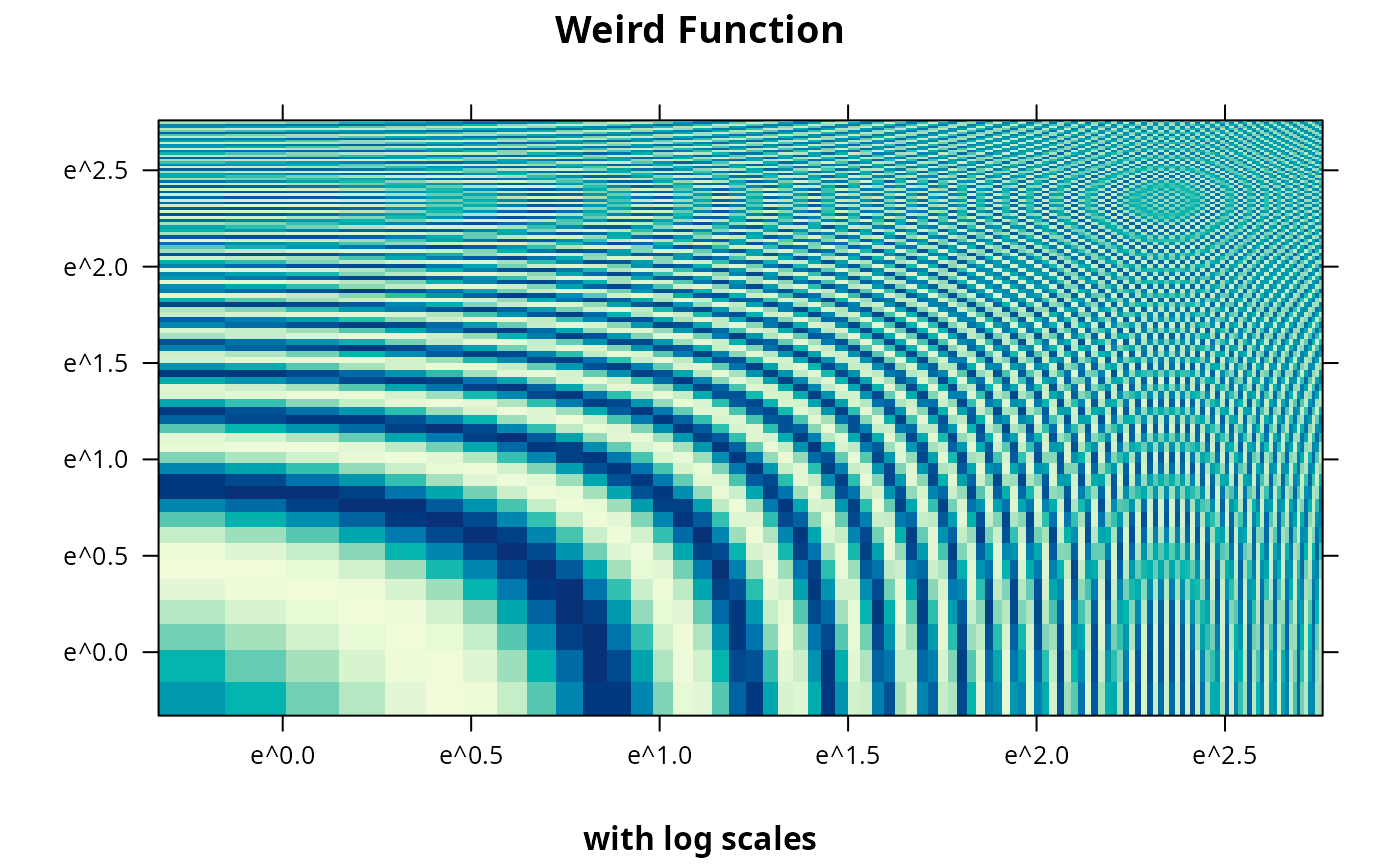
x <- seq(pi/4, 5 * pi, length.out = 100)
y <- seq(pi/4, 5 * pi, length.out = 100)
r <- as.vector(sqrt(outer(x^2, y^2, "+")))
grid <- expand.grid(x=x, y=y)
grid$z <- cos(r^2) * exp(-r/(pi^3))
levelplot(z ~ x * y, grid, cuts = 50, scales=list(log="e"), xlab="",
          ylab="", main="Weird Function", sub="with log scales",
          colorkey = FALSE, region = TRUE)

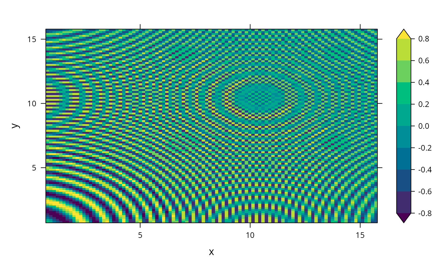
## triangular end-points in color key, with a title
levelplot(z ~ x * y, grid, col.regions = hcl.colors(10),
          at = c(-Inf, seq(-0.8, 0.8, by = 0.2), Inf))


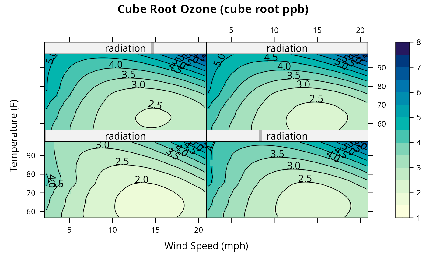
#S-PLUS example
require(stats)
attach(environmental)
ozo.m <- loess((ozone^(1/3)) ~ wind * temperature * radiation,
       parametric = c("radiation", "wind"), span = 1, degree = 2)
w.marginal <- seq(min(wind), max(wind), length.out = 50)
t.marginal <- seq(min(temperature), max(temperature), length.out = 50)
r.marginal <- seq(min(radiation), max(radiation), length.out = 4)
wtr.marginal <- list(wind = w.marginal, temperature = t.marginal,
        radiation = r.marginal)
grid <- expand.grid(wtr.marginal)
grid[, "fit"] <- c(predict(ozo.m, grid))
contourplot(fit ~ wind * temperature | radiation, data = grid,
            cuts = 10, region = TRUE,
            xlab = "Wind Speed (mph)",
            ylab = "Temperature (F)",
            main = "Cube Root Ozone (cube root ppb)")

detach()