The Relaxed Lasso

Introduction

In this vignette, we describe how the glmnet package can be used to fit the relaxed lasso.

The idea of the relaxed lasso is to take a glmnet fitted object, and then for each lambda, refit the variables in the active set without any penalization. This gives the “relaxed” fit. (We note that there have been other definitions of a relaxed fit, but this is the one we prefer.) This could of course be done for elastic net fits as well as lasso. However, if the number of variables gets too close to the sample size $N$ , the relaxed path will be truncated. Furthermore, for binomial and other nonlinear generalized linear models (GLMs) convergence can be an issue with our current implementation if the number of variables is too large, and perversely if the relaxed fit is too strong.

Suppose the glmnet fitted linear predictor at $\lambda$ is $\hat\eta_\lambda(x)$ and the relaxed version is $\tilde\eta_\lambda(x)$ . We also allow for shrinkage between the two: $\tilde \eta_{\lambda,\gamma}=(1-\gamma)\tilde \eta_\lambda(x)+\gamma\hat\eta_\lambda(x).$

$\gamma\in[0,1]$ is an additional tuning parameter which can be selected by cross-validation (CV). The debiasing will potentially improve prediction performance, and CV will typically select a model with a smaller number of variables.

This procedure is very competitive with forward-stepwise and best-subset regression, and has a considerable speed advantage when the number of variables is large. This is especially true for best-subset, but even so for forward stepwise. The latter has to plod through the variables one-at-a-time, while glmnet will just plunge in and find a good active set.

Further details on this form of relaxed fitting can be found in Hastie, Tibshirani, and Tibshirani (2017); more information on glmnet and elastic-net model in general is given in Friedman, Hastie, and Tibshirani (2010), Simon et al. (2011), Tibshirani et al. (2012), and Simon, Friedman, and Hastie (2013).

Simple relaxed fitting

We demonstrate the most basic relaxed lasso fit as a first example. We load some pre-generated data and fit the relaxed lasso on it by calling glmnet with relax = TRUE:

library(glmnet)

## Loading required package: Matrix

## Loaded glmnet 4.1-9

data(QuickStartExample)
x <- QuickStartExample$x
y <- QuickStartExample$y
fit <- glmnet(x, y, relax = TRUE)
print(fit)

## 
## Call:  glmnet(x = x, y = y, relax = TRUE) 
## Relaxed
## 
##    Df  %Dev %Dev R  Lambda
## 1   0  0.00   0.00 1.63100
## 2   2  5.53  58.90 1.48600
## 3   2 14.59  58.90 1.35400
## 4   2 22.11  58.90 1.23400
## 5   2 28.36  58.90 1.12400
## 6   2 33.54  58.90 1.02400
## 7   4 39.04  76.56 0.93320
## 8   5 45.60  80.59 0.85030
## 9   5 51.54  80.59 0.77470
## 10  6 57.35  87.99 0.70590
....

In addition to the three columns usually printed for glmnet objects (Df, %Dev and Lambda), there is an extra column %Dev R (R stands for “relaxed”) which is the percent deviance explained by the relaxed fit. This is always higher than its neighboring column, which is the percent deviance exaplined for the penalized fit (on the training data). Notice that when the Df stays the same, the %Dev R does not change, since this typically means the active set is the same. (The code is also smart enough to only fit such models once, so in the truncated display shown, 9 lasso models are fit, but only 4 relaxed fits are computed).

The fit object is of class "relaxed", which inherits from class "glmnet". Hence, the usual plot method for "glmnet" objects can be used. The code below demonstrates some additional flexibility that "relaxed" objects have for plotting.

par(mfrow = c(1, 3), mar=c(4,4,5.5,1))
plot(fit, main = "gamma = 1")
plot(fit, gamma = 0.5, main = "gamma = 0.5")
plot(fit, gamma = 0, main = "gamma = 0")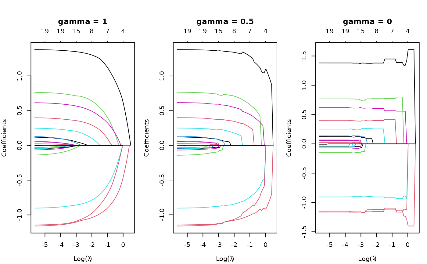

gamma = 1 is the traditional glmnet fit (also relax = FALSE, the default), gamma = 0 is the unpenalized fit, and gamma = 0.5 is a mixture of the two (at the coefficient level, and hence also the linear predictors).

We can also select gamma using cv.glmnet, which by default uses the 5 values c(0, 0.25, 0.5, 0.75, 1). This returns an object of class "cv.relaxed".

set.seed(1)
cfit <- cv.glmnet(x, y, relax = TRUE)
plot(cfit)

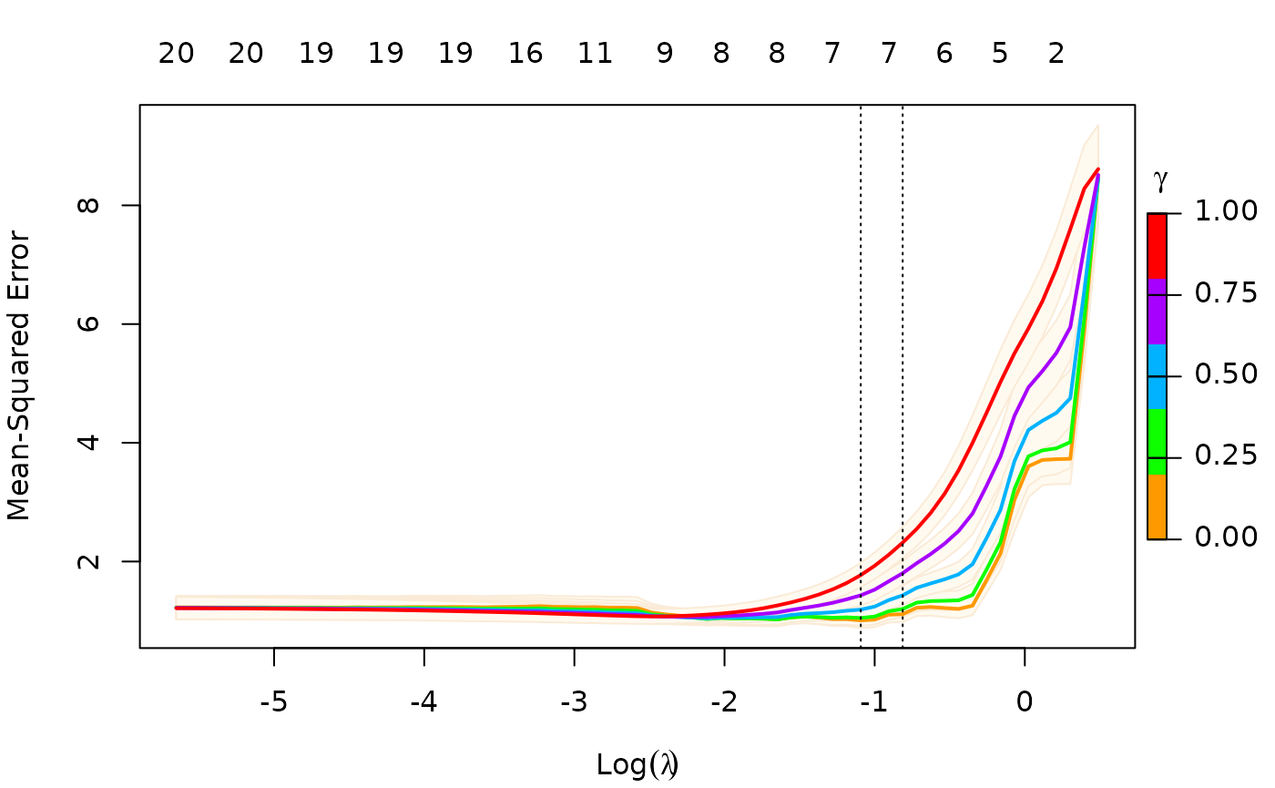
To remove the shading of the standard error bands, pass se.bands = FALSE:

plot(cfit, se.bands = FALSE)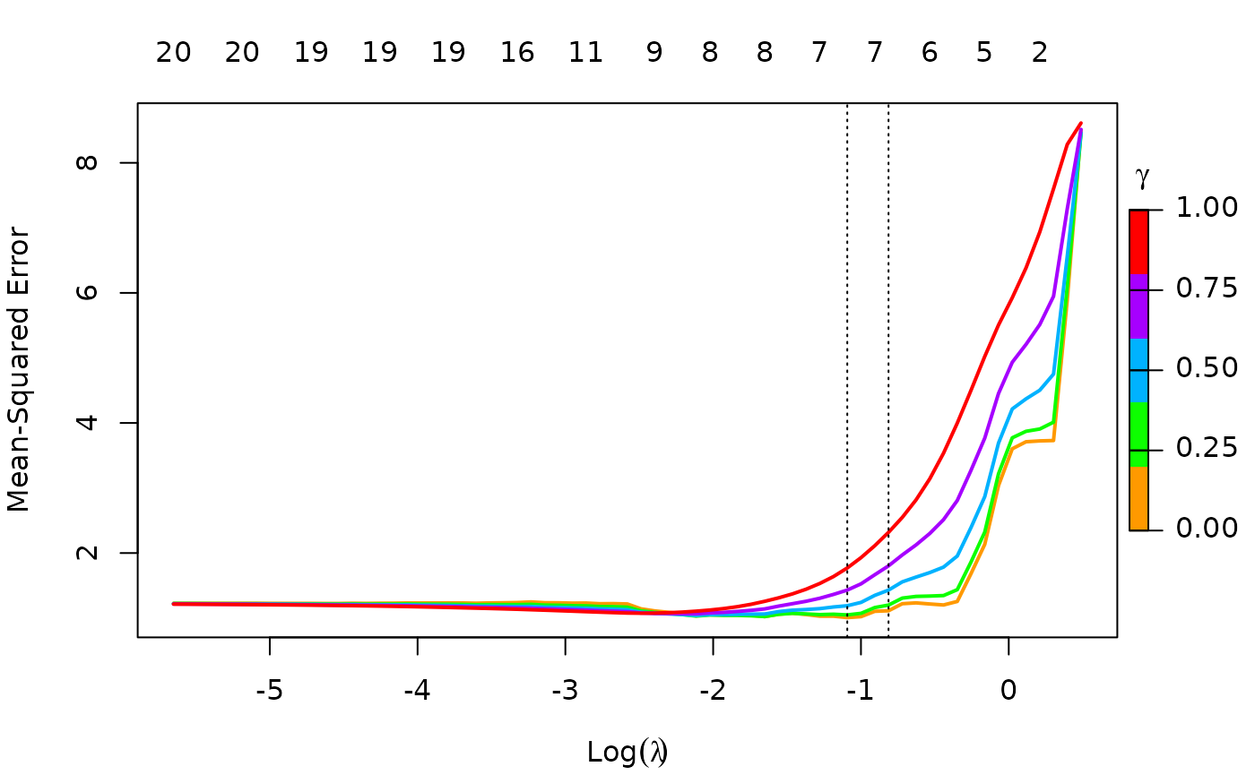

As with regular "cv.glmnet" objects, you can make predictions from a relaxed CV object. Just as the s option (for lambda) admits two special strings "lambda.1se" and "lambda.min" for special values of lambda, the gamma option admits two special strings "gamma.1se" and "gamma.min" for special values of gamma. For example, the code below makes predictions for newx at the lambda and gamma values that has the smallest CV error:

predict(cfit, newx = x[1:5, ], s = "lambda.min", gamma = "gamma.min")

##      lambda.min
## [1,] -1.6281344
## [2,]  2.6698376
## [3,]  0.3511622
## [4,]  1.9185110
## [5,]  1.5664349

Printing class "cv.relaxed" objects gives some basic information on the cross-validation:

print(cfit)

## 
## Call:  cv.glmnet(x = x, y = y, relax = TRUE) 
## 
## Measure: Mean-Squared Error 
## 
##     Gamma Index Lambda Index Measure     SE Nonzero
## min     0     1 0.3354    18   1.007 0.1269       7
## 1se     0     1 0.4433    15   1.112 0.1298       7

More details on relaxed fitting

While we only demonstrate relaxed fits for the default Gaussian family, any of the families fit by glmnet can also be fit with the relaxed option.

Although glmnet has a relax option, you can also fit relaxed lasso models by post-processing a glmnet object with the relax.glmnet function.

fit <- glmnet(x,y)
fitr <- relax.glmnet(fit, x = x, y = y)

This will rarely need to be done; one use case is if the original fit took a long time, and the user wants to avoid refitting it. Note that the arguments are named in the call in order for them to be passed correctly via the ... argument in relax.glmnet.

As mentioned, a "relaxed" object inherits from class "glmnet". Apart from the class modification, it has an additional component named relaxed which is itself a glmnet object, but with the relaxed coefficients. The default behavior of extractor functions like predict and coef, as well as plot will be to present results from the glmnet fit, unless a value of gamma is given different from the default value gamma = 1 (see the plots above). The print method gives additional info on the relaxed fit.

Likewise, a cv.relaxed object inherits from class cv.glmnet. Here the predict method by default uses the optimal relaxed fit; if predictions from the CV-optimal original glmnet fit are desired, one can directly use predict.cv.glmnet. Similarly, use print to print information for cross-validation on the relaxed fit, and print.cv.glmnet for information on the cross-validation for the original glmnet fit.

print(cfit)

## 
## Call:  cv.glmnet(x = x, y = y, relax = TRUE) 
## 
## Measure: Mean-Squared Error 
## 
##     Gamma Index Lambda Index Measure     SE Nonzero
## min     0     1 0.3354    18   1.007 0.1269       7
## 1se     0     1 0.4433    15   1.112 0.1298       7

print.cv.glmnet(cfit)

## 
## Call:  cv.glmnet(x = x, y = y, relax = TRUE) 
## 
## Measure: Mean-Squared Error 
## 
##      Lambda Index Measure     SE Nonzero
## min 0.08307    33   1.075 0.1251       9
## 1se 0.15933    26   1.175 0.1374       8

Possible convergence issues for relaxed fits

glmnet itself is used to fit the relaxed fits by using a single value of zero for lambda. However, for nonlinear models such as family = "binomial", family = "multinomial" and family="poisson", there can be convergence issues. This is because glmnet does not do step size optimization, rather relying on the pathwise fit to stay in the “quadratic” zone of the log-likelihood. We have an optional path = TRUE option for relax.glmnet, which actually fits a regurized path toward the lambda = 0 solution, and thus avoids the issue. The default is path = FALSE since this option adds to the computing time.

Application to forward stepwise regression

One use case for a relaxed fit is as a faster version of forward stepwise regression. With a large number p of variables, forward stepwise regression can be tedious. On the other hand, because the lasso solves a convex problem, it can plunge in and identify good candidate sets of variables over 100 values of lambda, even though p could be in the tens of thousands. In a case like this, one can have cv.glmnet do the selection of variables.

fitr <- cv.glmnet(x, y, gamma = 0, relax = TRUE)
plot(fitr)

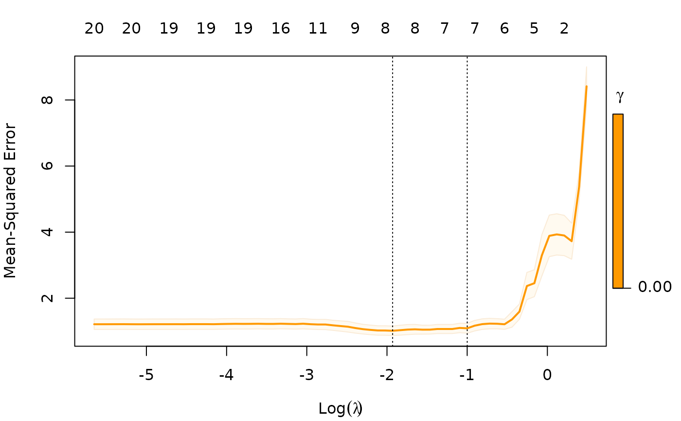
Notice that we only allow gamma = 0, so in this case we are not considering the blended fits.

References

Friedman, Jerome, Trevor Hastie, and Robert Tibshirani. 2010. “Regularization Paths for Generalized Linear Models via Coordinate Descent.” Journal of Statistical Software, Articles 33 (1): 1–22. https://doi.org/10.18637/jss.v033.i01.

Hastie, Trevor, Robert Tibshirani, and Ryan Tibshirani. 2017. “Extended Comparisons of Best Subset Selection, Forward Stepwise Selection, and the Lasso.”

Simon, Noah, Jerome Friedman, and Trevor Hastie. 2013. “A Blockwise Descent Algorithm for Group-Penalized Multiresponse and Multinomial Regression.” https://doi.org/10.48550/arXiv.1311.6529.

Simon, Noah, Jerome Friedman, Trevor Hastie, and Robert Tibshirani. 2011. “Regularization Paths for Cox’s Proportional Hazards Model via Coordinate Descent.” Journal of Statistical Software, Articles 39 (5): 1–13. https://doi.org/10.18637/jss.v039.i05.

Tibshirani, Robert, Jacob Bien, Jerome Friedman, Trevor Hastie, Noah Simon, Jonathan Taylor, and Ryan Tibshirani. 2012. “Strong Rules for Discarding Predictors in Lasso-Type Problems.” Journal of the Royal Statistical Society: Series B (Statistical Methodology) 74 (2): 245–66. https://doi.org/10.1111/j.1467-9868.2011.01004.x.

Trevor Hastie

Balasubramanian Narasimhan