An Introduction to glmnet

Trevor Hastie

Junyang Qian

Kenneth Tay

July 02, 2025

Introduction

Glmnet is a package that fits generalized linear and similar models via penalized maximum likelihood. The regularization path is computed for the lasso or elastic net penalty at a grid of values (on the log scale) for the regularization parameter lambda. The algorithm is extremely fast, and can exploit sparsity in the input matrix x. It fits linear, logistic and multinomial, poisson, and Cox regression models. It can also fit multi-response linear regression, generalized linear models for custom families, and relaxed lasso regression models. The package includes methods for prediction and plotting, and functions for cross-validation.

The authors of glmnet are Jerome Friedman, Trevor Hastie, Rob Tibshirani, Balasubramanian Narasimhan, Kenneth Tay and Noah Simon, with contribution from Junyang Qian, and the R package is maintained by Trevor Hastie. A MATLAB version of glmnet is maintained by Junyang Qian, and a Python version by B. Balakumar (although both are a few versions behind).

This vignette describes basic usage of glmnet in R. There are additional vignettes that should be useful:

• “Regularized Cox Regression” describes how to fit regularized Cox models for survival data with glmnet.
• “GLM family functions in glmnet” describes how to fit custom generalized linear models (GLMs) with the elastic net penalty via the family argument.
• “The Relaxed Lasso” describes how to fit relaxed lasso regression models using the relax argument.

glmnet solves the problem

$$\min_{\beta_0,\beta} \frac{1}{N} \sum_{i=1}^{N} w_i l(y_i,\beta_0+\beta^T x_i) + \lambda\left[(1-\alpha)\|\beta\|_2^2/2 + \alpha \|\beta\|_1\right],$$

over a grid of values of $\lambda$ covering the entire range of possible solutions. Here $l(y_i,\eta_i)$ is the negative log-likelihood contribution for observation $i$; e.g. for the Gaussian case it is $\frac{1}{2}(y_i-\eta_i)^2$. The elastic net penalty is controlled by $\alpha$, and bridges the gap between lasso regression ($\alpha=1$, the default) and ridge regression ($\alpha=0$). The tuning parameter $\lambda$ controls the overall strength of the penalty.

It is known that the ridge penalty shrinks the coefficients of correlated predictors towards each other while the lasso tends to pick one of them and discard the others. The elastic net penalty mixes these two: if predictors are correlated in groups, an $\alpha=0.5$ tends to either select or leave out the entire group of features. This is a higher level parameter, and users might pick a value upfront or experiment with a few different values. One use of $\alpha$ is for numerical stability; for example, the elastic net with $\alpha = 1 - \epsilon$ for some small $\epsilon > 0$ performs much like the lasso, but removes any degeneracies and wild behavior caused by extreme correlations.

The glmnet algorithms use cyclical coordinate descent, which successively optimizes the objective function over each parameter with others fixed, and cycles repeatedly until convergence. The package also makes use of the strong rules for efficient restriction of the active set. Due to highly efficient updates and techniques such as warm starts and active-set convergence, our algorithms can compute the solution path very quickly.

The code can handle sparse input-matrix formats, as well as range constraints on coefficients. The core of glmnet is a set of Fortran subroutines, which make for very fast execution.

The theory and algorithms in this implementation are described in Friedman, Hastie, and Tibshirani (2010), Simon et al. (2011), Tibshirani et al. (2012) and Simon, Friedman, and Hastie (2013).

Installation

Like many other R packages, the simplest way to obtain glmnet is to install it directly from CRAN. Type the following command in R console:

install.packages("glmnet", repos = "https://cran.us.r-project.org")

Users may change the repos argument depending on their locations and preferences. Other arguments such as the directories to install the packages at can be altered in the command. For more details, see help(install.packages). Alternatively, users can download the package source from CRAN and type Unix commands to install it to the desired location.

Quick Start

The purpose of this section is to give users a general sense of the package. We will briefly go over the main functions, basic operations and outputs. After this section, users may have a better idea of what functions are available, which ones to use, or at least where to seek help.

First, we load the glmnet package:

library(glmnet)

## Loading required package: Matrix

## Loaded glmnet 4.1-9

The default model used in the package is the Guassian linear model or “least squares”, which we will demonstrate in this section. We load a set of data created beforehand for illustration:

data(QuickStartExample)
x <- QuickStartExample$x
y <- QuickStartExample$y

The command loads an input matrix x and a response vector y from this saved R data archive.

We fit the model using the most basic call to glmnet.

fit <- glmnet(x, y)

fit is an object of class glmnet that contains all the relevant information of the fitted model for further use. We do not encourage users to extract the components directly. Instead, various methods are provided for the object such as plot, print, coef and predict that enable us to execute those tasks more elegantly.

We can visualize the coefficients by executing the plot method:

plot(fit)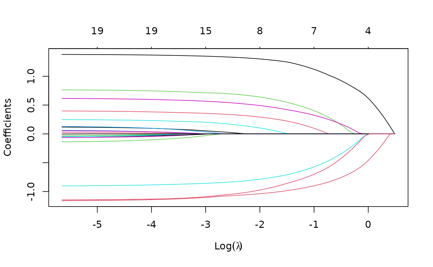

Each curve corresponds to a variable. It shows the path of its coefficient against the $\ell_1$-norm of the whole coefficient vector as $\lambda$ varies. The axis above indicates the number of nonzero coefficients at the current $\lambda$, which is the effective degrees of freedom (df) for the lasso. Users may also wish to annotate the curves: this can be done by setting label = TRUE in the plot command.

A summary of the glmnet path at each step is displayed if we just enter the object name or use the print function:

print(fit)

## 
## Call:  glmnet(x = x, y = y) 
## 
##    Df  %Dev  Lambda
## 1   0  0.00 1.63100
## 2   2  5.53 1.48600
## 3   2 14.59 1.35400
## 4   2 22.11 1.23400
## 5   2 28.36 1.12400
## 6   2 33.54 1.02400
....

It shows from left to right the number of nonzero coefficients (Df), the percent (of null) deviance explained (%dev) and the value of $\lambda$ (Lambda). Although glmnet fits the model for 100 values of lambda by default, it stops early if %dev does not change sufficently from one lambda to the next (typically near the end of the path.) Here we have truncated the prinout for brevity.

We can obtain the model coefficients at one or more $\lambda$’s within the range of the sequence:

coef(fit, s = 0.1)

## 21 x 1 sparse Matrix of class "dgCMatrix"
##                       s0
## (Intercept)  0.150928072
## V1           1.320597195
## V2           .          
## V3           0.675110234
## V4           .          
## V5          -0.817411518
## V6           0.521436671
## V7           0.004829335
....

(Why s and not lambda? In case we want to allow one to specify the model size in other ways in the future.) Users can also make predictions at specific $\lambda$’s with new input data:

set.seed(29)
nx <- matrix(rnorm(5 * 20), 5, 20)
predict(fit, newx = nx, s = c(0.1, 0.05))

##              s0         s1
## [1,] -4.3067990 -4.5979456
## [2,] -4.1244091 -4.3447727
## [3,] -0.1133939 -0.1859237
## [4,]  3.3458748  3.5270269
## [5,] -1.2366422 -1.2772955

The function glmnet returns a sequence of models for the users to choose from. In many cases, users may prefer the software to select one of them. Cross-validation is perhaps the simplest and most widely used method for that task. cv.glmnet is the main function to do cross-validation here, along with various supporting methods such as plotting and prediction.

cvfit <- cv.glmnet(x, y)

cv.glmnet returns a cv.glmnet object, a list with all the ingredients of the cross-validated fit. As with glmnet, we do not encourage users to extract the components directly except for viewing the selected values of $\lambda$. The package provides well-designed functions for potential tasks. For example, we can plot the object:

plot(cvfit)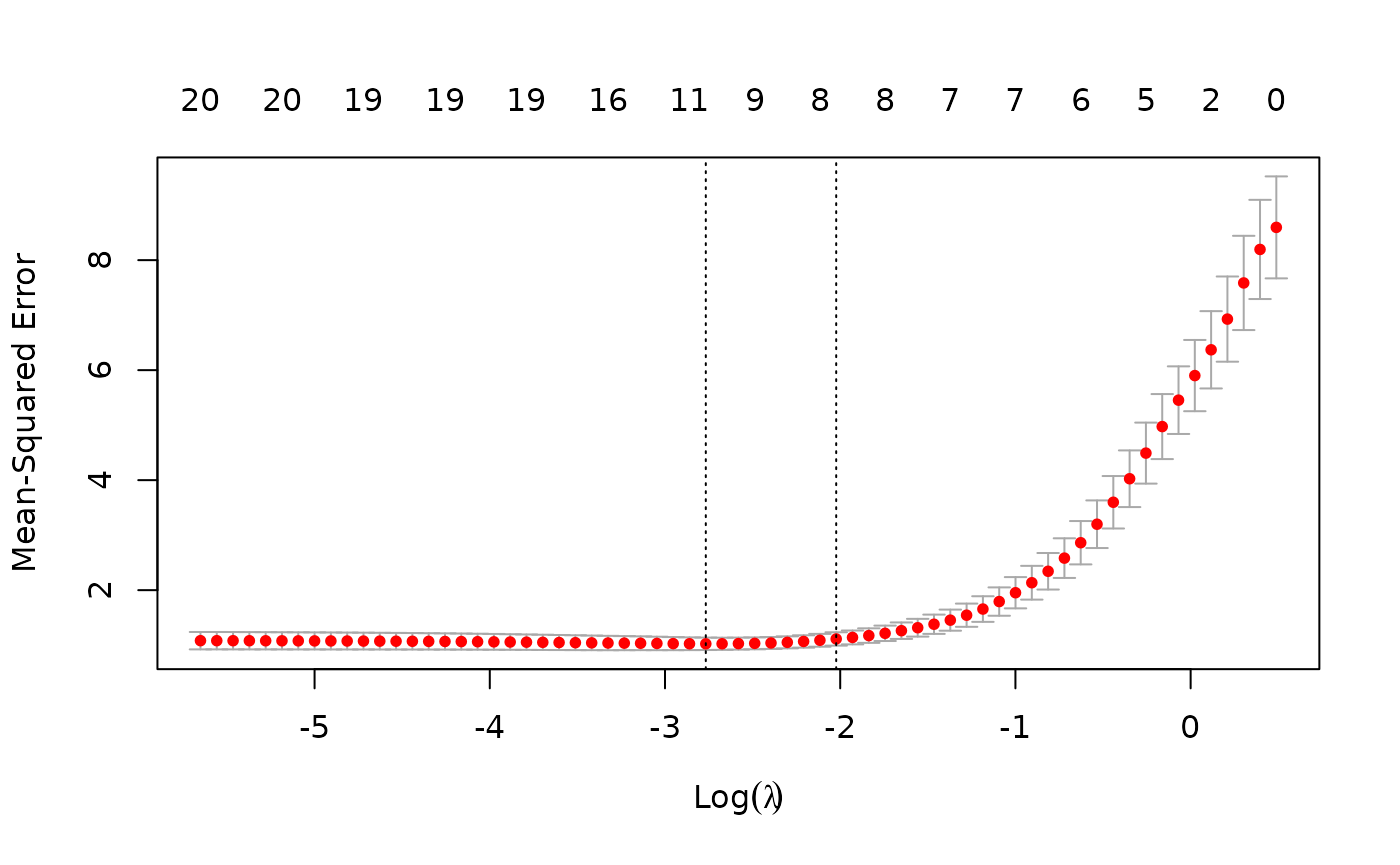

This plots the cross-validation curve (red dotted line) along with upper and lower standard deviation curves along the $\lambda$ sequence (error bars). Two special values along the $\lambda$ sequence are indicated by the vertical dotted lines. lambda.min is the value of $\lambda$ that gives minimum mean cross-validated error, while lambda.1se is the value of $\lambda$ that gives the most regularized model such that the cross-validated error is within one standard error of the minimum.

We can use the following code to get the value of lambda.min and the model coefficients at that value of $\lambda$:

cvfit$lambda.min

## [1] 0.06284188

coef(cvfit, s = "lambda.min")

## 21 x 1 sparse Matrix of class "dgCMatrix"
##                       s0
## (Intercept)  0.145832036
## V1           1.340981414
## V2           .          
## V3           0.708347140
## V4           .          
## V5          -0.848087765
## V6           0.554823782
## V7           0.038519738
....

To get the corresponding values at lambda.1se, simply replace lambda.min with lambda.1se above, or omit the s argument, since lambda.1se is the default.

Note that the coefficients are represented in the sparse matrix format. This is because the solutions along the regularization path are often sparse, and hence it is more efficient in time and space to use a sparse format. If you prefer non-sparse format, pipe the output through as.matrix().

Predictions can be made based on the fitted cv.glmnet object as well. The code below gives predictions for the new input matrix newx at lambda.min:

predict(cvfit, newx = x[1:5,], s = "lambda.min")

##      lambda.min
## [1,] -1.3574653
## [2,]  2.5776672
## [3,]  0.5846421
## [4,]  2.0280562
## [5,]  1.5780633

This concludes glmnet 101. With the tools introduced so far, users are able to fit the entire elastic net family, including ridge regression, using squared-error loss. There are many more arguments in the package that give users a great deal of flexibility. To learn more, move on to later sections.

Linear Regression: family = "gaussian" (default)

"gaussian" is the default family argument for the function glmnet. Suppose we have observations $x_i \in \mathbb{R}^p$ and the responses $y_i \in \mathbb{R}, i = 1, \ldots, N$. The objective function for the Gaussian family is $$\min_{(\beta_0, \beta) \in \mathbb{R}^{p+1}}\frac{1}{2N} \sum_{i=1}^N (y_i -\beta_0-x_i^T \beta)^2+\lambda \left[ (1-\alpha)\|\beta\|_2^2/2 + \alpha\|\beta\|_1\right],$$ where $\lambda \geq 0$ is a complexity parameter and $0 \leq \alpha \leq 1$ is a compromise between ridge regression ($\alpha = 0$) and lasso regression ($\alpha = 1$).

glmnet applies coordinate descent to solve the problem. Specifically, suppose we have current estimates $\tilde{\beta_0}$ and $\tilde{\beta}_\ell$$\forall \ell\in 1,\ldots,p$. By computing the gradient at $\beta_j = \tilde{\beta}_j$ and simple calculus, the update is $$\tilde{\beta}_j \leftarrow \frac{S(\frac{1}{N}\sum_{i=1}^N x_{ij}(y_i-\tilde{y}_i^{(j)}),\lambda \alpha)}{1+\lambda(1-\alpha)},$$ where $\tilde{y}_i^{(j)} = \tilde{\beta}_0 + \sum_{\ell \neq j} x_{i\ell} \tilde{\beta}_\ell$, and $S(z, \gamma)$ is the soft-thresholding operator with value $\text{sign}(z)(|z|-\gamma)_+$.

This formula above applies when the x variables are standardized to have unit variance (the default); it is slightly more complicated when they are not. Note that for family = "gaussian", glmnet standardizes $y$ to have unit variance before computing its lambda sequence (and then unstandardizes the resulting coefficients). If you wish to reproduce or compare results with other software, it is best to supply a standardized $y$ first (Using the “1/N” variance formula).

Commonly used function arguments

glmnet provides various arguments for users to customize the fit: we introduce some commonly used arguments here. (For more information, type ?glmnet.)

• alpha is for the elastic net mixing parameter $\alpha$, with range $\alpha \in [0,1]$. $\alpha = 1$ is lasso regression (default) and $\alpha = 0$ is ridge regression.

• weights is for the observation weights, default is 1 for each observation. (Note: glmnet rescales the weights internally to sum to N, the sample size.)

• nlambda is the number of $\lambda$ values in the sequence (default is 100).

• lambda can be provided if the user wants to specify the lambda sequence, but typical usage is for the program to construct the lambda sequence on its own. When automatically generated, the $\lambda$ sequence is determined by lambda.max and lambda.min.ratio. The latter is the ratio of smallest value of the generated $\lambda$ sequence (say lambda.min) to lambda.max. The program generates nlambda values linear on the log scale from lambda.max down to lambda.min. lambda.max is not user-specified but is computed from the input $x$ and $y$: it is the smallest value for lambda such that all the coefficients are zero. For alpha = 0 (ridge) lambda.max would be $\infty$: in this case we pick a value corresponding to a small value for alpha close to zero.)

• standardize is a logical flag for x variable standardization prior to fitting the model sequence. The coefficients are always returned on the original scale. Default is standardize = TRUE.

As an example, we set $\alpha = 0.2$ (more like a ridge regression), and give double weight to the latter half of the observations. We set nlambda to 20 so that the model fit is only compute for 20 values of $\lambda$. In practice, we recommend nlambda to be 100 (default) or more. In most cases, it does not come with extra cost because of the warm-starts used in the algorithm, and for nonlinear models leads to better convergence properties.

wts <-  c(rep(1,50), rep(2,50))
fit <- glmnet(x, y, alpha = 0.2, weights = wts, nlambda = 20)

We can then print the glmnet object:

print(fit)

## 
## Call:  glmnet(x = x, y = y, weights = wts, alpha = 0.2, nlambda = 20) 
## 
##    Df  %Dev Lambda
## 1   0  0.00 7.9390
## 2   4 17.89 4.8890
## 3   7 44.45 3.0110
## 4   7 65.67 1.8540
## 5   8 78.50 1.1420
## 6   9 85.39 0.7033
## 7  10 88.67 0.4331
## 8  11 90.25 0.2667
## 9  14 91.01 0.1643
## 10 17 91.38 0.1012
## 11 17 91.54 0.0623
## 12 17 91.60 0.0384
## 13 19 91.63 0.0236
## 14 20 91.64 0.0146
## 15 20 91.64 0.0090
## 16 20 91.65 0.0055
## 17 20 91.65 0.0034

This displays the call that produced the object fit and a three-column matrix with columns Df (the number of nonzero coefficients), %dev (the percent deviance explained) and Lambda (the corresponding value of $\lambda$). (The digits argument can used to specify significant digits in the printout.)

Here the actual number of $\lambda$’s is less than that specified in the call. This is because of the algorithm’s stopping criteria. According to the default internal settings, the computations stop if either the fractional change in deviance down the path is less than $10^{-5}$ or the fraction of explained deviance reaches $0.999$. From the last few lines of the output, we see the fraction of deviance does not change much and therefore the computation ends before the all 20 models are fit. The internal parameters governing the stopping criteria can be changed. For details, see the Appendix section or type help(glmnet.control).

Predicting and plotting with glmnet objects

We can extract the coefficients and make predictions for a glmnet object at certain values of $\lambda$. Two commonly used arguments are:

• s for specifiying the value(s) of $\lambda$ at which to extract coefficients/predictions.

• exact for indicating whether the exact values of coefficients are desired or not. If exact = TRUE and predictions are to be made at values of s not included in the original fit, these values of s are merged with object$lambda and the model is refit before predictions are made. If exact = FALSE (default), then the predict function uses linear interpolation to make predictions for values of s that do not coincide with lambdas used in the fitting algorithm.

Here is a simple example illustrating the use of both these function arguments:

fit <- glmnet(x, y)
any(fit$lambda == 0.5)  # 0.5 not in original lambda sequence

## [1] FALSE

coef.apprx <- coef(fit, s = 0.5, exact = FALSE)
coef.exact <- coef(fit, s = 0.5, exact = TRUE, x=x, y=y)
cbind2(coef.exact[which(coef.exact != 0)], 
       coef.apprx[which(coef.apprx != 0)])

##            [,1]       [,2]
## [1,]  0.2613110  0.2613110
## [2,]  1.0055470  1.0055473
## [3,]  0.2677140  0.2677134
## [4,] -0.4476485 -0.4476475
## [5,]  0.2379287  0.2379283
## [6,] -0.8230862 -0.8230865
## [7,] -0.5553678 -0.5553675

The left and right columns show the coefficients for exact = TRUE and exact = FALSE respectively. (For brevity we only show the non-zero coefficients.) We see from the above that 0.5 is not in the sequence and that hence there are some small differences in coefficient values. Linear interpolation is usually accurate enough if there are no special requirements. Notice that with exact = TRUE we have to supply by named argument any data that was used in creating the original fit, in this case x and y.

Users can make predictions from the fitted glmnet object. In addition to the arguments in coef, the primary argument is newx, a matrix of new values for x at which predictions are desired. The type argument allows users to choose the type of prediction returned:

• “link” returns the fitted values (i.e. $\hat\beta_0 + x_i^T\hat\beta$)

• “response” gives the same output as “link” for “gaussian” family.

• “coefficients” returns the model codfficients.

• “nonzero” retuns a list of the indices of the nonzero coefficients for each value of s.

For example, the following code gives the fitted values for the first 5 observations at $\lambda = 0.05$:

predict(fit, newx = x[1:5,], type = "response", s = 0.05)

##              s0
## [1,] -1.3362652
## [2,]  2.5894245
## [3,]  0.5872868
## [4,]  2.0977222
## [5,]  1.6436280

If multiple values of s are supplied, a matrix of predictions is produced. If no value of s is supplied, a matrix of predictions is supplied, with columns corresponding to all the lambdas used in the fit.

We can plot the fitted object as in the Quick Start section. Here we walk through more arguments for the plot function. The xvar argument allows users to decide what is plotted on the x-axis. xvar allows three measures: “norm” for the $\ell_1$-norm of the coefficients (default), “lambda” for the log-lambda value and “dev” for %deviance explained. Users can also label the curves with the variable index numbers simply by setting label = TRUE.

For example, let’s plot fit against the log-lambda value and with each curve labeled:

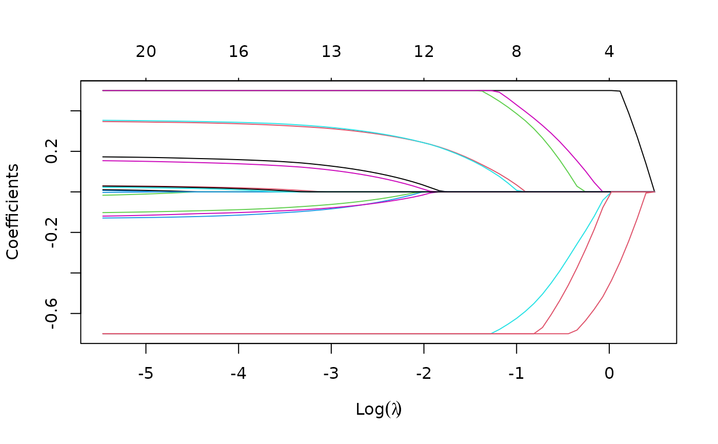
plot(fit, xvar = "lambda", label = TRUE)

Now when we plot against %deviance we get a very different picture. This is percent deviance explained on the training data, and is a measure of complexity of the model. We see that toward the end of the path, %deviance is not changing much but the coefficients are “blowing up” a bit. This enables us focus attention on the parts of the fit that matter. This will especially be true for other models, such as logistic regression.

plot(fit, xvar = "dev", label = TRUE)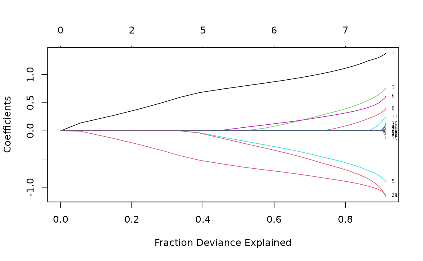

Cross-validation

K-fold cross-validation can be performed using the cv.glmnet function. In addition to all the glmnet parameters, cv.glmnet has its special parameters including nfolds (the number of folds), foldid (user-supplied folds), and type.measure(the loss used for cross-validation):

• “deviance” or “mse” for squared loss, and

• “mae” uses mean absolute error.

As an example,

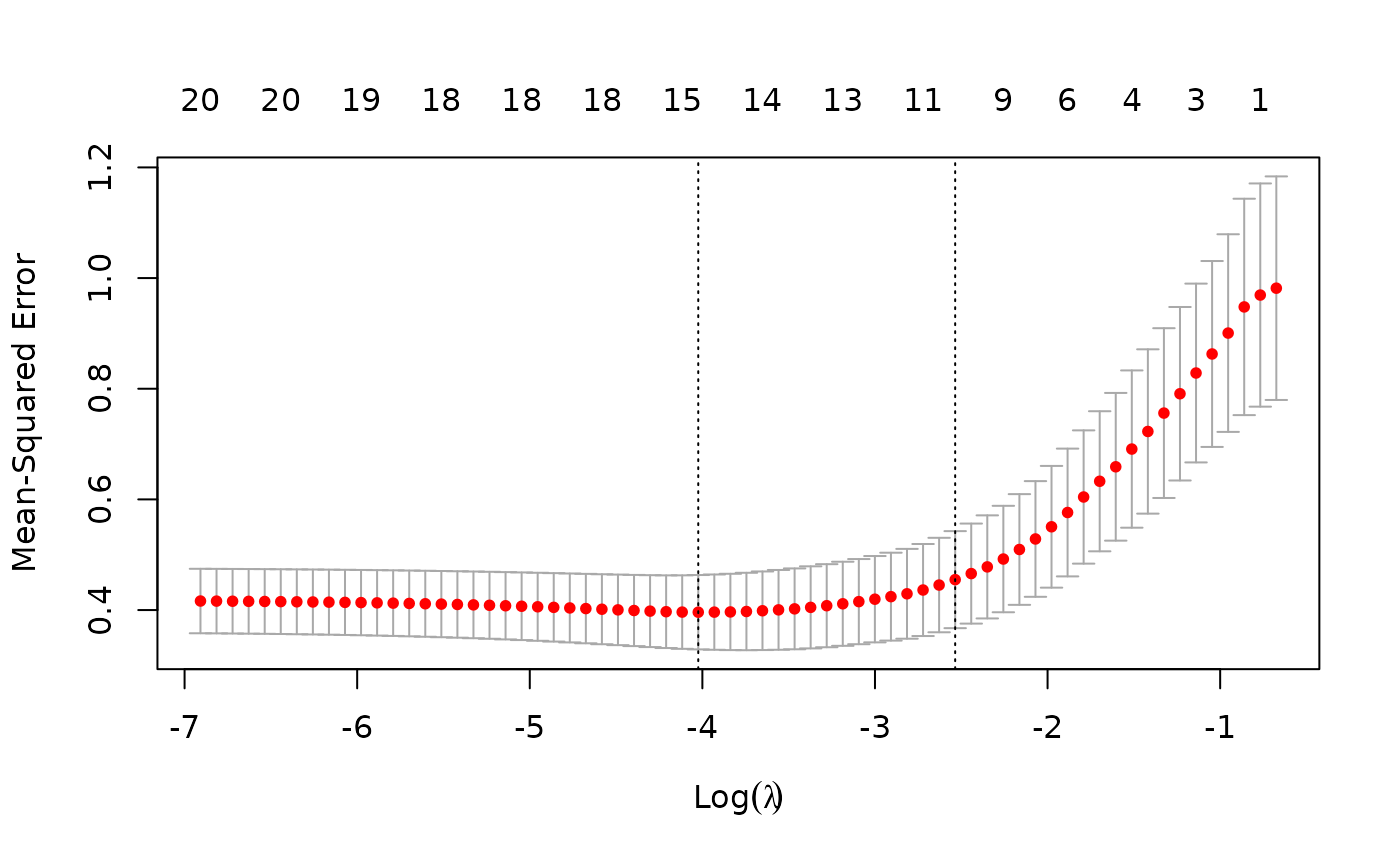
cvfit <- cv.glmnet(x, y, type.measure = "mse", nfolds = 20)

does 20-fold cross-validation based on mean squared error criterion (the default for “gaussian” family). Printing the resulting object gives some basic information on the cross-validation performed:

print(cvfit)

## 
## Call:  cv.glmnet(x = x, y = y, type.measure = "mse", nfolds = 20) 
## 
## Measure: Mean-Squared Error 
## 
##      Lambda Index Measure     SE Nonzero
## min 0.07569    34   1.063 0.1135       9
## 1se 0.14517    27   1.164 0.1297       8

cv.glmnet also supports parallel computing. To make it work, users must register parallel beforehand. We give a simple example of comparison here. Unfortunately, the package doMC is not available on Windows platforms (it is on others), so we cannot run the code here, but we present timing information recorded during one of our test runs.

library(doMC)
registerDoMC(cores = 2)
X <- matrix(rnorm(1e4 * 200), 1e4, 200)
Y <- rnorm(1e4)

system.time(cv.glmnet(X, Y))

##    user  system elapsed 
##   2.440   0.080   2.518

system.time(cv.glmnet(X, Y, parallel = TRUE))

##    user  system elapsed 
##   2.450   0.157   1.567

As suggested from the above, parallel computing can significantly speed up the computation process especially for large-scale problems.

The coef and predict methods for cv.glmnet objects are similar to those for a glmnet object, except that two special strings are also supported by s (the values of $\lambda$ requested):

• “lambda.min”: the $\lambda$ at which the smallest MSE is achieved.

• “lambda.1se”: the largest $\lambda$ at which the MSE is within one standard error of the smallest MSE (default).

cvfit$lambda.min

## [1] 0.07569327

predict(cvfit, newx = x[1:5,], s = "lambda.min")

##      lambda.min
## [1,] -1.3638848
## [2,]  2.5713428
## [3,]  0.5729785
## [4,]  1.9881422
## [5,]  1.5179882

coef(cvfit, s = "lambda.min")

## 21 x 1 sparse Matrix of class "dgCMatrix"
##                      s0
## (Intercept)  0.14867414
## V1           1.33377821
## V2           .         
## V3           0.69787701
## V4           .         
## V5          -0.83726751
## V6           0.54334327
## V7           0.02668633
....

Users can explicitly control the fold that each observation is assigned to via the foldid argument. This is useful, for example, in using cross-validation to select a value for $\alpha$:

foldid <- sample(1:10, size = length(y), replace = TRUE)
cv1  <- cv.glmnet(x, y, foldid = foldid, alpha = 1)
cv.5 <- cv.glmnet(x, y, foldid = foldid, alpha = 0.5)
cv0  <- cv.glmnet(x, y, foldid = foldid, alpha = 0)

There are no built-in plot functions to put them all on the same plot, so we are on our own here:

par(mfrow = c(2,2))
plot(cv1); plot(cv.5); plot(cv0)
plot(log(cv1$lambda)   , cv1$cvm , pch = 19, col = "red",
     xlab = "log(Lambda)", ylab = cv1$name)
points(log(cv.5$lambda), cv.5$cvm, pch = 19, col = "grey")
points(log(cv0$lambda) , cv0$cvm , pch = 19, col = "blue")
legend("topleft", legend = c("alpha= 1", "alpha= .5", "alpha 0"),
       pch = 19, col = c("red","grey","blue"))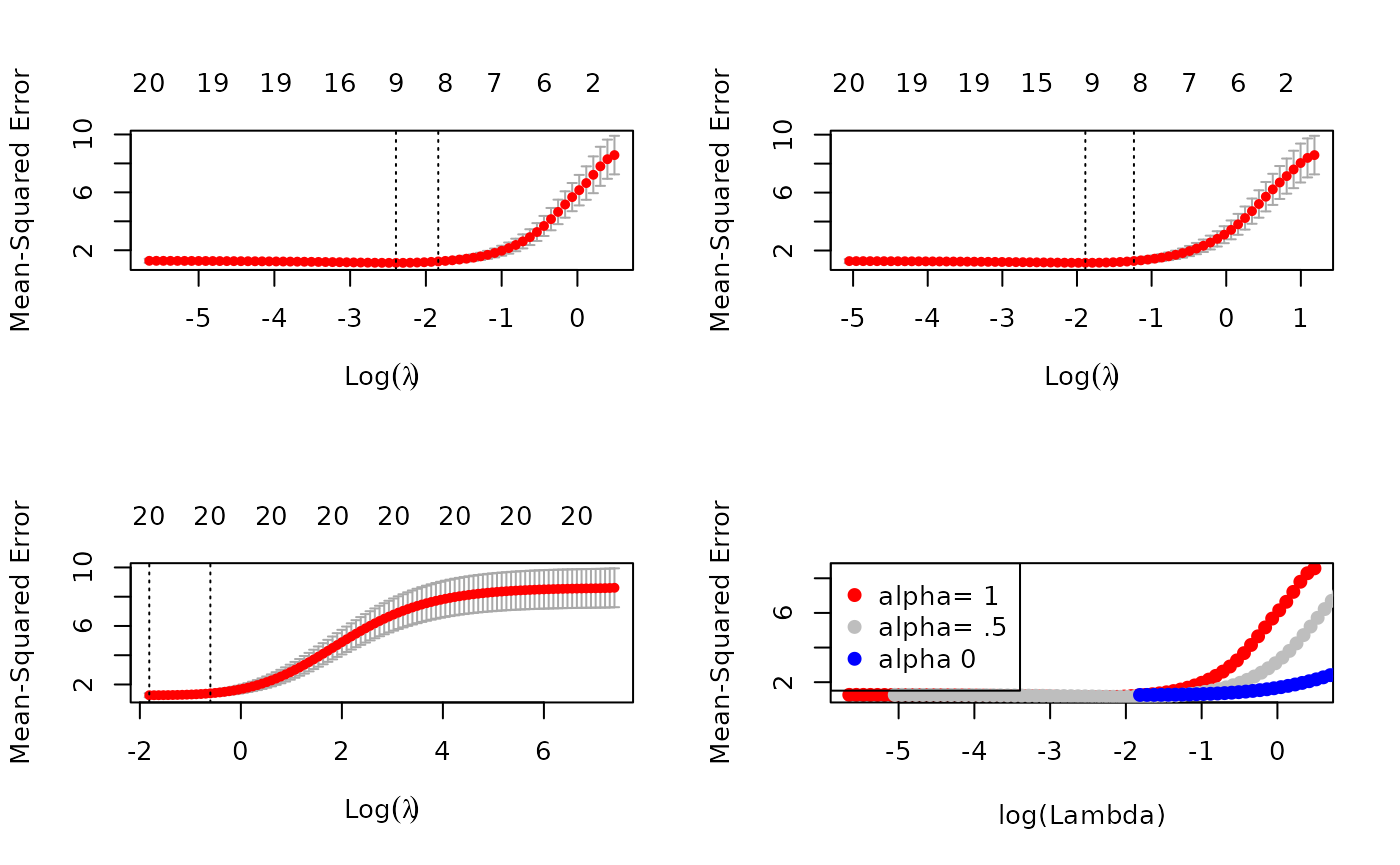

We see that the lasso (alpha=1) does about the best here. We also see that the range of lambdas used differs with alpha.

Other function arguments

In this section we breifly describe some other useful arguments when calling glmnet: upper.limits, lower.limits, penalty.factor, exclude and intercept.

Suppose we want to fit our model but limit the coefficients to be bigger than -0.7 and less than 0.5. This can be achieved by specifying the upper.limits and lower.limits arguments:

tfit <- glmnet(x, y, lower.limits = -0.7, upper.limits = 0.5)
plot(tfit)

Often we want the coefficients to be positive: to do so, we just need to specify lower.limits = 0. (Note, the lower limit must be no bigger than zero, and the upper limit no smaller than zero.) These bounds can be a vector, with different values for each coefficient. If given as a scalar, the same number gets recycled for all.

The penalty.factor argument allows users to apply separate penalty factors to each coefficient. This is very useful when we have prior knowledge or preference over the variables. Specifically, if $v_j$ denotes the penalty factor for the $j$th variable, the penalty term becomes $$\lambda \sum_{j=1}^p \boldsymbol{v_j} P_\alpha(\beta_j) = \lambda \sum_{j=1}^p \boldsymbol{v_j} \left[ (1-\alpha)\frac{1}{2} \beta_j^2 + \alpha |\beta_j| \right].$$

The default is 1 for each coefficient, i.e. coefficients are penalized equally. Note that any variable with penalty.factor equal to zero is not penalized at all! This is useful in the case where some variables are always to be included unpenalized in the model, such as the demographic variables sex and age in medical studies. Note the penalty factors are internally rescaled to sum to nvars, the number of variables in the given x matrix.

Here is an example where we set the penalty factors for variables 1, 3 and 5 to be zero:

p.fac <- rep(1, 20)
p.fac[c(1, 3, 5)] <- 0
pfit <- glmnet(x, y, penalty.factor = p.fac)
plot(pfit, label = TRUE)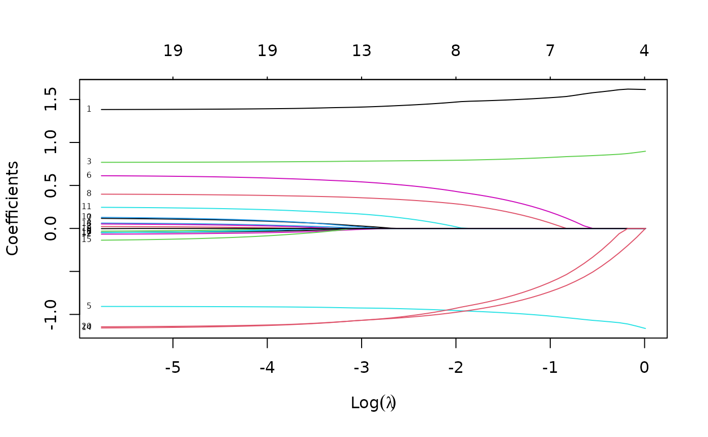

We see from the labels that the three variables with zero penalty factors always stay in the model, while the others follow typical regularization paths and shrunk to zero eventually.

exclude allows one to block certain variables from being the model at all. Of course, one could simply subset these out of x, but sometimes exclude is more useful, since it returns a full vector of coefficients, just with the excluded ones set to zero.

The intercept argument allows the user to decide if an intercept should be included in the model or not (it is never penalized). The default is intercept = TRUE. If intercept = FALSE the intercept is forced to be zero.

Linear Regression: family = "mgaussian" (multi-response)

The multi-response Gaussian family is useful when there are a number of (correlated) responses, also known as the “multi-task learning” problem. Here, a variable is either included in the model for all the responses, or excluded for all the responses. Most of the arguments for this family are the same as that for family = "gaussian", so we focus on the differences with the single response model.

As the name suggests, the response $y$ is not a vector but a matrix of quantitative responses. As a result, the coefficients at each value of lambda are also a matrix.

glmnet solves the problem $$\min_{(\beta_0, \beta) \in \mathbb{R}^{(p+1)\times K}}\frac{1}{2N} \sum_{i=1}^N \|y_i -\beta_0-\beta^T x_i\|^2_F+\lambda \left[ (1-\alpha)\|\beta\|_F^2/2 + \alpha\sum_{j=1}^p\|\beta_j\|_2\right].$$ Here $\beta_j$ is the $j$th row of the $p\times K$ coefficient matrix $\beta$, and we replace the absolute penalty on each single coefficient by a group-lasso penalty on each coefficient $K$-vector $\beta_j$ for a single predictor (i.e. column of the x matrix). The group lasso penalty behaves like the lasso, but on the whole group of coefficients for each response: they are either all zero, or else none are zero, but are shrunk by an amount depending on $\lambda$.

We use a set of data generated beforehand for illustration. We fit a regularized multi-response Gaussian model to the data, with an object mfit returned.

data(MultiGaussianExample)
x <- MultiGaussianExample$x
y <- MultiGaussianExample$y
mfit <- glmnet(x, y, family = "mgaussian")

The standardize.response argument is only for mgaussian family. If standardize.response = TRUE, the response variables are standardized (default is FALSE).

As before, we can use the plot method to visualize the coefficients:

plot(mfit, xvar = "lambda", label = TRUE, type.coef = "2norm")

Note that we set type.coef = "2norm". Under this setting, a single curve is plotted per variable, with value equal to the $\ell_2$ norm of the variable’s coefficient vector. The default setting is type.coef = "coef", where a coefficient plot is created for each response (multiple figures). xvar and label are two other arguments which have the same functionality as in the single-response case.

We can extract the coefficients and make predictions at requested values of $\lambda$ by using the coef and predict methods respectively, as before. Here is an example of a predict call:

predict(mfit, newx = x[1:5,], s = c(0.1, 0.01))

## , , 1
## 
##              y1         y2         y3       y4
## [1,] -4.7106263 -1.1634574  0.6027634 3.740989
## [2,]  4.1301735 -3.0507968 -1.2122630 4.970141
## [3,]  3.1595229 -0.5759621  0.2607981 2.053976
## [4,]  0.6459242  2.1205605 -0.2252050 3.146286
## [5,] -1.1791890  0.1056262 -7.3352965 3.248370
## 
## , , 2
## 
##              y1         y2         y3       y4
## [1,] -4.6415158 -1.2290282  0.6118289 3.779521
## [2,]  4.4712843 -3.2529658 -1.2572583 5.266039
## [3,]  3.4735228 -0.6929231  0.4684037 2.055574
## [4,]  0.7353311  2.2965083 -0.2190297 2.989371
## [5,] -1.2759930  0.2892536 -7.8259206 3.205211

The prediction result is saved in a three-dimensional array with the first two dimensions being the prediction matrix for each response variable and the third corresponding to the response variables.

Logistic Regression: family = "binomial"

Logistic regression is a widely-used model when the response is binary. Suppose the response variable takes values in $\mathcal{G}=\{1,2\}$. Denote $y_i = I(g_i=1)$. We model

$$\mbox{Pr}(G=2|X=x)=\frac{e^{\beta_0+\beta^Tx}}{1+e^{\beta_0+\beta^Tx}},$$

which can be written in the following form:

$$\log\frac{\mbox{Pr}(G=2|X=x)}{\mbox{Pr}(G=1|X=x)}=\beta_0+\beta^Tx,$$ the so-called “logistic” or log-odds transformation.

The objective function for logistic regression is the penalized negative binomial log-likelihood, and is $$\min_{(\beta_0, \beta) \in \mathbb{R}^{p+1}} -\left[\frac{1}{N} \sum_{i=1}^N y_i \cdot (\beta_0 + x_i^T \beta) - \log (1+e^{(\beta_0+x_i^T \beta)})\right] + \lambda \big[ (1-\alpha)\|\beta\|_2^2/2 + \alpha\|\beta\|_1\big].$$ Logistic regression is often plagued with degeneracies when $p > N$ and exhibits wild behavior even when $N$ is close to $p$; the elastic net penalty alleviates these issues, and regularizes and selects variables as well.

We use a “proximal Newton” algorithm for optimizing this criterion. This makes repeated use of a quadratic approximation to the log-likelihood, and then weighted coordinate descent on the resulting penalized weighted least-squares problem. These constitute an outer and inner loop, also known as iteratively reweighted penalized least squares.

For illustration purposes, we load the pre-generated input matrix x and the response vector y from the data file. The input matrix $x$ is the same as for other families. For binomial logistic regression, the response variable $y$ should be either a binary vector, a factor with two levels, or a two-column matrix of counts or proportions. The latter is useful for grouped binomial data, or in applications where we have “soft” class membership, such as occurs in the EM algorithm.

data(BinomialExample)
x <- BinomialExample$x
y <- BinomialExample$y

Other optional arguments of glmnet for binomial regression are almost same as those for Gaussian family. Don’t forget to set family option to “binomial”:

fit <- glmnet(x, y, family = "binomial")

As before, we can print and plot the fitted object, extract the coefficients at specific $\lambda$’s and also make predictions. For plotting, the optional arguments such as xvar and label work in the same way as for family = "gaussian". Prediction is a little different for family = "binomial", mainly in the function argument type:

• “link” gives the linear predictors.

• “response” gives the fitted probabilities.

• “class” produces the class label corresponding to the maximum probability.

As with family = "gaussian", “coefficients” computes the coefficients at values of s and “nonzero” retuns a list of the indices of the nonzero coefficients for each value of s. Note that the results (“link”, “response”, “coefficients”, “nonzero”) are returned only for the class corresponding to the second level of the factor response.

In the following example, we make prediction of the class labels at $\lambda = 0.05, 0.01$.

predict(fit, newx = x[1:5,], type = "class", s = c(0.05, 0.01))

##      s0  s1 
## [1,] "0" "0"
## [2,] "1" "1"
## [3,] "1" "1"
## [4,] "0" "0"
## [5,] "1" "1"

For logistic regression, cv.glmnet has similar arguments and usage as Gaussian. nfolds, weights, lambda, parallel are all available to users. There are some differences in type.measure: “deviance” and “mse” do not both mean squared loss. Rather,

• “mse” uses squared loss.

• “deviance” uses actual deviance.

• “mae” uses mean absolute error.

• “class” gives misclassification error.

• “auc” (for two-class logistic regression ONLY) gives area under the ROC curve.

For example, the code below uses misclassification error as the criterion for 10-fold cross-validation:

cvfit <- cv.glmnet(x, y, family = "binomial", type.measure = "class")

As before, we can plot the object and show the optimal values of $\lambda$.

plot(cvfit)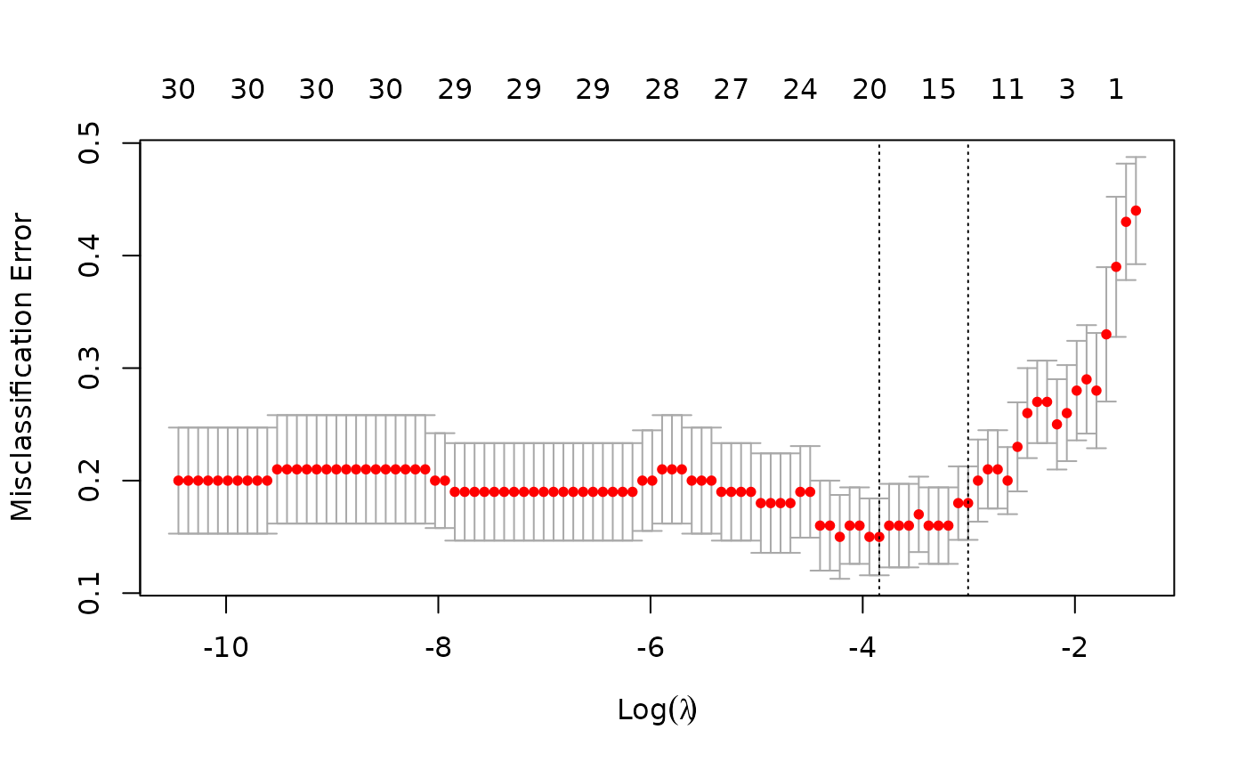

cvfit$lambda.min

## [1] 0.02140756

cvfit$lambda.1se

## [1] 0.04945423

coef and predict for the cv.glmnet object for family = "binomial" are simliar to the Gaussian case and we omit the details.

Like other generalized linear models, glmnet allows for an “offset”. This is a fixed vector of $N$ numbers that is added into the linear predictor. For example, you may have fitted some other logistic regression using other variables (and data), and now you want to see if the present variables can add further predictive power. To do this, you can use the predicted logit from the other model as an offset in the glmnet call. Offsets are also useful in Poisson models, which we discuss later.

Multinomial Regression: family = "multinomial"

The multinomial model extends the binomial when the number of classes is more than two. Suppose the response variable has $K$ levels ${\cal G}=\{1,2,\ldots,K\}$. Here we model $$\mbox{Pr}(G=k|X=x)=\frac{e^{\beta_{0k}+\beta_k^Tx}}{\sum_{\ell=1}^Ke^{\beta_{0\ell}+\beta_\ell^Tx}}.$$ There is a linear predictor for each class!

Let ${Y}$ be the $N \times K$ indicator response matrix, with elements $y_{i\ell} = I(g_i=\ell)$. Then the elastic net penalized negative log-likelihood function becomes $$\ell(\{\beta_{0k},\beta_{k}\}_1^K) = -\left[\frac{1}{N} \sum_{i=1}^N \Big(\sum_{k=1}^Ky_{il} (\beta_{0k} + x_i^T \beta_k)- \log \big(\sum_{\ell=1}^K e^{\beta_{0\ell}+x_i^T \beta_\ell}\big)\Big)\right] +\lambda \left[ (1-\alpha)\|\beta\|_F^2/2 + \alpha\sum_{j=1}^p\|\beta_j\|_q\right].$$ Here we really abuse notation! $\beta$ is a $p\times K$ matrix of coefficients. $\beta_k$ refers to the $k$th column (for outcome category $k$), and $\beta_j$ the $j$th row (vector of $K$ coefficients for variable $j$). The last penalty term is $\|\beta_j\|_q$. We support two options for $q$: $q\in \{1,2\}$. When $q=1$, this is a lasso penalty on each of the parameters. When $q=2$, this is a grouped-lasso penalty on all the $K$ coefficients for a particular variable, which makes them all be zero or nonzero together.

The standard Newton algorithm can be tedious here. Instead, for $q=1$ we use a so-called partial Newton algorithm by making a partial quadratic approximation to the log-likelihood, allowing only $(\beta_{0k}, \beta_k)$ to vary for a single class at a time. For each value of $\lambda$, we first cycle over all classes indexed by $k$, computing each time a partial quadratic approximation about the parameters of the current class. Then, the inner procedure is almost the same as for the binomial case. When $q=2$, we use a different approach that we will not explain here.

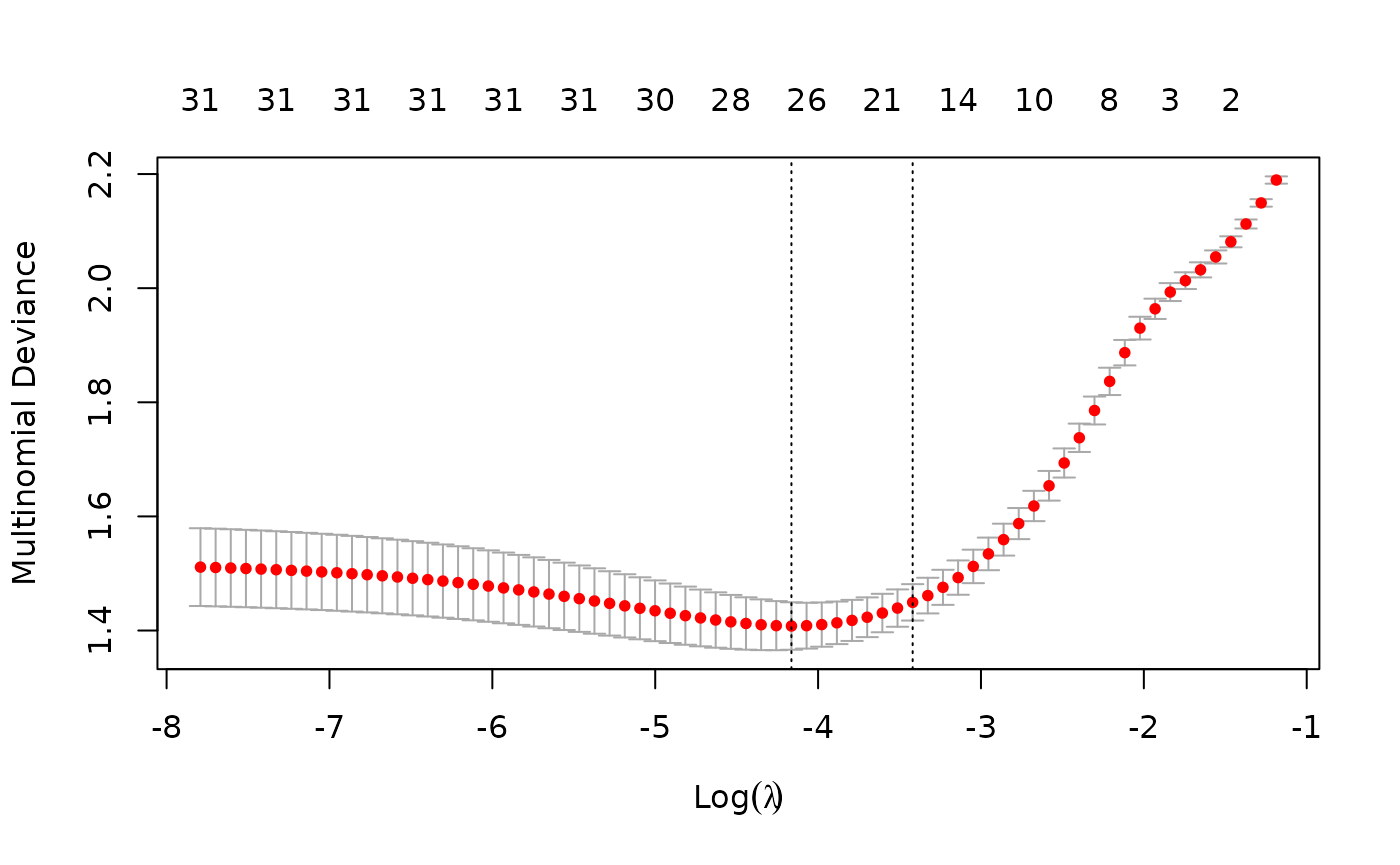
For the family = "multinomial" case, usage is similar to that for family = "binomial". In this section we describe the differences. First, we load a set of generated data:

data(MultinomialExample)
x <- MultinomialExample$x
y <- MultinomialExample$y

The response variable can be a nc >= 2 level factor, or an nc-column matrix of counts or proportions. Internally glmnet will make the rows of this matrix sum to 1, and absorb the total mass into the weight for that observation. offset should be a nobs x nc matrix if one is provided.

A special option for multinomial regression is type.multinomial, which allows the usage of a grouped lasso penalty ($q = 2$) if type.multinomial = "grouped". The default is type.multinomial = "ungrouped" ($q = 1$).

fit <- glmnet(x, y, family = "multinomial", type.multinomial = "grouped")
plot(fit, xvar = "lambda", label = TRUE, type.coef = "2norm")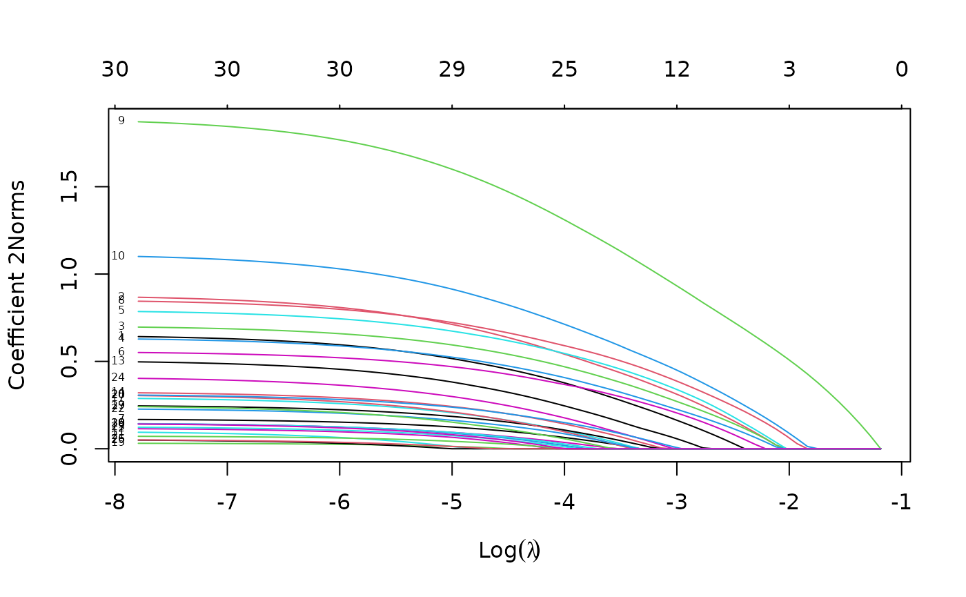

For the plot method, the function arguments are xvar, label and type.coef, in addition to other ordinary graphical parameters. xvar and label are the same as other families while type.coef is only for multinomial regression and multi-response Gaussian model. It can produce a figure of coefficients for each response variable if type.coef = "coef" or a figure showing the $\ell_2$-norm in one figure if type.coef = "2norm".

We can also do cross-validation and plot the returned object. Note that although type.multinomial is not a named argument in cv.glmnet, in fact any argument that can be passed to glmnet is valid in the argument list of cv.glmnet. Such arguments are passed via the ... argument directly to the calls to glmnet inside the cv.glmnet function.

cvfit <- cv.glmnet(x, y, family = "multinomial", type.multinomial = "grouped")
plot(cvfit)

Users may wish to predict at the optimally selected $\lambda$:

predict(cvfit, newx = x[1:10,], s = "lambda.min", type = "class")

##       1  
##  [1,] "3"
##  [2,] "2"
##  [3,] "2"
##  [4,] "3"
##  [5,] "1"
##  [6,] "3"
##  [7,] "3"
##  [8,] "1"
##  [9,] "1"
## [10,] "2"

Poisson Regression: family = "poisson"

Poisson regression is used to model count data under the assumption of Poisson error, or otherwise non-negative data where the mean and variance are proportional. Like the Gaussian and binomial models, the Poisson distribution is a member of the exponential family of distributions. We usually model its positive mean on the log scale: $\log \mu(x) = \beta_0+\beta' x$.

The log-likelihood for observations $\{x_i,y_i\}_1^N$ is given by $$l(\beta|X, Y) = \sum_{i=1}^N \left(y_i (\beta_0+\beta^T x_i) - e^{\beta_0+\beta^Tx_i}\right).$$ As before, we optimize the penalized log-likelihood: $$\min_{\beta_0,\beta} -\frac1N l(\beta|X, Y) + \lambda \left((1-\alpha) \sum_{i=1}^N \beta_i^2/2 +\alpha \sum_{i=1}^N |\beta_i|\right).$$

glmnet uses an outer Newton loop and an inner weighted least-squares loop (as in logistic regression) to optimize this criterion.

First, we load a pre-generated set of Poisson data:

data(PoissonExample)
x <- PoissonExample$x
y <- PoissonExample$y

We apply the function glmnet with family = "poisson":

fit <- glmnet(x, y, family = "poisson")

The optional input arguments of glmnet for "poisson" family are similar to those for other families.

offset is a particularly useful argument for Poisson models. When dealing with rate data in Poisson models, the counts collected are often based on different exposures such as length of time observed, area and years. A poisson rate $\mu(x)$ is relative to a unit exposure time, so if an observation $y_i$ was exposed for $E_i$ units of time, then the expected count would be $E_i\mu(x)$, and the log mean would be $\log(E_i)+\log(\mu(x))$. In a case like this, we would supply an offset $\log(E_i)$ for each observation. Hence offset is a vector of length $N$ that is included in the linear predictor. (Warning: if offset is supplied in glmnet, offsets must also also be supplied to predict via the newoffset argument to make reasonable predictions.)

Again, we plot the coefficients to have a first sense of the result.

plot(fit)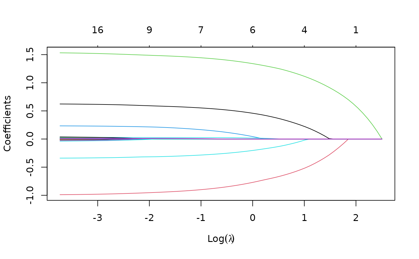

As before, we can extract the coefficients and make predictions at certain $\lambda$’s using coef and predict respectively. The optional input arguments are similar to those for other families. For the predict method, the argument type has the same meaning as that for family = "binomial", except that “response” gives the fitted mean (rather than fitted probabilities in the binomial case). For example, we can do the following:

coef(fit, s = 1)

## 21 x 1 sparse Matrix of class "dgCMatrix"
##                      s0
## (Intercept)  0.61123371
## V1           0.45819758
## V2          -0.77060709
## V3           1.34015128
## V4           0.04350500
....

predict(fit, newx = x[1:5,], type = "response", s = c(0.1,1))

##              s0         s1
## [1,]  2.4944232  4.4263365
## [2,] 10.3513120 11.0586174
## [3,]  0.1179704  0.1781626
## [4,]  0.9713412  1.6828778
## [5,]  1.1133472  1.9934537

We may also use cross-validation to find the optimal $\lambda$’s and thus make inferences.

cvfit <- cv.glmnet(x, y, family = "poisson")

Options are almost the same as the Gaussian family except that for type.measure:

• “deviance” (default) gives the deviance.
• “mse” is for mean squared error.
• “mae” is for mean absolute error.

Cox Regression: family = "cox"

The Cox proportional hazards model is commonly used for the study of the relationship beteween predictor variables and survival time. We have another vignette (“Regularized Cox Regression”) dedicated solely to fitting regularized Cox models with the glmnet package; please consult that vignette for details.

Programmable GLM families: family = family()

Since version 4.0, glmnet has the facility to fit any GLM family by specifying a family object, as used by stats::glm. For these more general families, the outer Newton loop is performed in R, while the inner elastic-net loop is performed in Fortran, for each value of lambda. The price for this generality is a small hit in speed. For details, see the vignette “GLM family functions in glmnet”

Assessing models on test data

Once we have fit a series of models using glmnet, we often assess their performance on a set of evaluation or test data. We usually go through the process of building a prediction matrix, deciding on the performance measure, and computing these measures for a series of values for lambda (and gamma for relaxed fits). glmnet provides three functions (assess.glmnet, roc.glmnet and confusion.glmnet) that make these tasks easier.

Performance measures

The function assess.glmnet computes the same performance measures produced by cv.glmnet, but on a validation or test dataset.

data(BinomialExample)
x <- BinomialExample$x
y <- BinomialExample$y
itrain <- 1:70
fit <- glmnet(x[itrain, ], y[itrain], family = "binomial", nlambda = 5)
assess.glmnet(fit, newx = x[-itrain, ], newy = y[-itrain])

## $deviance
##        s0        s1        s2        s3        s4 
## 1.3877348 0.8612331 1.7948439 3.0335905 3.6930687 
## attr(,"measure")
## [1] "Binomial Deviance"
## 
## $class
##        s0        s1        s2        s3        s4 
## 0.4666667 0.1666667 0.2333333 0.1666667 0.1666667 
## attr(,"measure")
## [1] "Misclassification Error"
## 
## $auc
## [1] 0.5000000 0.9062500 0.8482143 0.8169643 0.8303571
## attr(,"measure")
## [1] "AUC"
## 
## $mse
##        s0        s1        s2        s3        s4 
## 0.5006803 0.2529304 0.3633411 0.3514574 0.3500440 
## attr(,"measure")
## [1] "Mean-Squared Error"
## 
## $mae
##        s0        s1        s2        s3        s4 
## 0.9904762 0.5114320 0.4597047 0.3928790 0.3767338 
## attr(,"measure")
## [1] "Mean Absolute Error"

This produces a list with all the measures suitable for a binomial model, computed for the entire sequence of lambdas in the fit object. Here the function identifies the model family from the fit object.

A second use case builds the prediction matrix before calling assess.glmnet:

pred <- predict(fit, newx = x[-itrain, ])
assess.glmnet(pred, newy = y[-itrain], family = "binomial")

Here we have to provide the family as an argument; the results (not shown) are the same. Users can see the various measures suitable for each family via

glmnet.measures()

## $gaussian
## [1] "mse" "mae"
## 
## $binomial
## [1] "deviance" "class"    "auc"      "mse"      "mae"     
## 
## $poisson
## [1] "deviance" "mse"      "mae"     
## 
## $cox
## [1] "deviance" "C"       
## 
## $multinomial
## [1] "deviance" "class"    "mse"      "mae"     
## 
## $mgaussian
## [1] "mse" "mae"
## 
## $GLM
## [1] "deviance" "mse"      "mae"

assess.glmnet can also take the result of cv.glmnet as input. In this case the predictions are made at the optimal values for the parameter(s).

cfit <- cv.glmnet(x[itrain, ], y[itrain], family = "binomial", nlambda = 30)
assess.glmnet(cfit, newx = x[-itrain, ], newy = y[-itrain])

## $deviance
## lambda.1se 
##  0.9482246 
## attr(,"measure")
## [1] "Binomial Deviance"
## 
## $class
## lambda.1se 
##        0.2 
## attr(,"measure")
## [1] "Misclassification Error"
....

This uses the default value of s = "lambda.1se", just like predict would have done. Users can provide additional arguments that get passed on to predict. For example, the code below shows the performance measures for s = "lambda.min":

assess.glmnet(cfit, newx = x[-itrain, ],newy = y[-itrain], s = "lambda.min")

## $deviance
## lambda.min 
##  0.8561849 
## attr(,"measure")
## [1] "Binomial Deviance"
## 
## $class
## lambda.min 
##  0.1666667 
## attr(,"measure")
## [1] "Misclassification Error"
....

Prevalidation

One interesting use case for assess.glmnet is to get the results of cross-validation using other measures. By specifying keep = TRUE in the cv.glmnet call, a matrix of prevalidated predictions are stored in the returned output as the fit.preval component. We can then use this component in the call to assess.glmnet:

cfit <- cv.glmnet(x, y, family = "binomial", keep = TRUE, nlambda = 30)
assess.glmnet(cfit$fit.preval, newy = y, family = "binomial")

## $deviance
##        s0        s1        s2        s3        s4        s5        s6        s7 
## 1.4131504 1.2947431 1.1887748 1.0940954 0.9903013 0.8999068 0.8407559 0.8075691 
##        s8        s9       s10       s11       s12       s13       s14       s15 
## 0.8053265 0.8302531 0.8783749 0.9490040 1.0501903 1.1733004 1.2947184 1.4200727 
##       s16       s17       s18       s19       s20       s21       s22       s23 
## 1.5596069 1.7098302 1.8594572 2.0060912 2.1283083 2.2510820 2.3757275 2.4799198 
##       s24       s25       s26       s27       s28       s29 
## 2.5765861 2.6589164 2.7143188 2.7634920 2.8119805 2.8404461 
## attr(,"measure")
## [1] "Binomial Deviance"
....

Users can verify that the first measure here deviance is identical to the component cvm on the cfit object.

ROC curves for binomial data

In the special case of binomial models, users often would like to see the ROC curve for validation or test data. Here the function roc.glmnet provides the goodies. Its first argument is as in assess.glmnet. Here we illustrate one use case, using the prevlidated CV fit.

cfit <- cv.glmnet(x, y, family = "binomial", type.measure = "auc", 
                  keep = TRUE)
rocs <- roc.glmnet(cfit$fit.preval, newy = y)

roc.glmnet returns a list of cross-validated ROC data, one for each model along the path. The code below demonstrates how one can plot the output. The first line identifies the lambda value giving the best area under the curve (AUC). Then we plot all the ROC curves in grey and the “winner” in red.

best <- cvfit$index["min",]
plot(rocs[[best]], type = "l")
invisible(sapply(rocs, lines, col="grey"))
lines(rocs[[best]], lwd = 2,col = "red")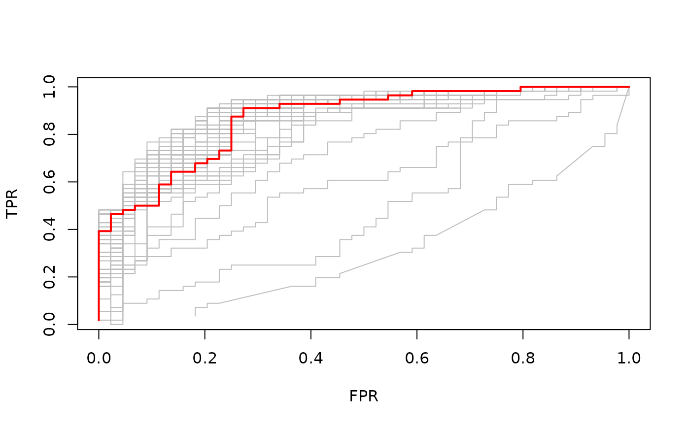

Confusion matrices for classification

For binomial and multinomial models, we often wish to examine the classification performance on new data. The function confusion.glmnet will do that for us.

data(MultinomialExample)
x <- MultinomialExample$x
y <- MultinomialExample$y
set.seed(101)
itrain <- sample(1:500, 400, replace = FALSE)
cfit <- cv.glmnet(x[itrain, ], y[itrain], family = "multinomial")
cnf <- confusion.glmnet(cfit, newx = x[-itrain, ], newy = y[-itrain])

confusion.glmnet produces a table of class “confusion.table” which inherits from class “table”, and we also provide a print method for it.

print(cnf)

##          True
## Predicted  1  2  3 Total
##     1     13  6  4    23
##     2      7 25  5    37
##     3      4  3 33    40
##     Total 24 34 42   100
## 
##  Percent Correct:  0.71

The first argument to confusion.glmnet should be a glmnet or cv.glmnet object (from which predictions can be made), or a matrix/array of predictions, such as the kept "fit.preval" component in the output of a cv.glmnet call with keep = TRUE. When a matrix/array of predictions is provided, we need to specify the family option, otherwise confusion can exist between “binomial” and “multinomial” prediction matrices.

When predictions for more than one model in the path is provided, confusion.glmnet returns a list of confusion tables. For example, the prevalidated predictions from cv.glmnet are for the whole lambda path, and so we are returned a list of confusion tables. In the code below, we identify and print the one achieving the smallest classification error.

cfit <- cv.glmnet(x, y, family = "multinomial", type = "class", keep = TRUE)
cnf <- confusion.glmnet(cfit$fit.preval, newy = y, family = "multinomial")
best <- cfit$index["min",]
print(cnf[[best]])

##          True
## Predicted   1   2   3 Total
##     1      76  22  14   112
##     2      39 129  23   191
##     3      27  23 147   197
##     Total 142 174 184   500
## 
##  Percent Correct:  0.704

Filtering variables

The exclude argument to glmnet accepts a vector of indices, indicating which variables should be excluded from the fit, i.e. get zeros for their coefficients. From version 4.1-2, the exclude argument can accept a function. The idea is that variables can be filtered based on some of their properties (e.g. too sparse) before any models are fit. When performing cross-validation (CV), this filtering should be done separately inside each fold of cv.glmnet.

Here is a typical filter function: it excludes variables that are more than 80% sparse.

filter <- function(x, ...) which(colMeans(x == 0) > 0.8)

This function gets invoked inside the call to glmnet, and uses the supplied x to generate the indices.

We give a simple example using this:

set.seed(101)
n <-500; p <- 50
x <- matrix(rnorm(n * p), n, p)
x[sample(seq(length(x)), 4 * n * p / 5)] <- 0
y <- rnorm(n) + x %*% (rnorm(p) / 5) > 0
excl <- filter(x)
print(excl)

##  [1]  4  5  6  7  8  9 11 15 22 23 24 25 26 27 28 29 33 35 36 40 42 46

fit.orig <- glmnet(x, y, family = "binomial", exclude = excl)
fit.new  <- glmnet(x, y, family = "binomial", exclude = filter)
all.equal(fit.orig, fit.new)

## [1] "Component \"call\": target, current do not match when deparsed"

The fits are the same (the call component is all that differs).

The nice thing with this approach is that cv.glmnet does the right thing: it applies the filter function separately to each training-fold x, and hence accounts for any bias that may be incurred by the filtering.

cvfit.filt <- cv.glmnet(x, y, family = "binomial", exclude = filter)

The most general form of the filter function is

filter <- function(x, y, weights, ...) {}

Yes, users can use y as well in their filtering criterion, and the observation weights if that makes sense. As we did above, some of the arguments can be omitted, but the ... must always be there. We will give some useful examples of filter functions a bit later.

An important point to note is that any other arguments in a user’s filter function are ignored. So, what we should if we want one or more additional parameters to guide the filtering, such as the choice of 0.8 in our filter function above? The safest way to achieve this is to write a filter generator function, that produces a filter function as its output. We give an example:

sparsity <- function(fraction = 0.7) {
  function(x, ...) which(colMeans(x == 0) > fraction)
}
sparsity(0.5)

## function (x, ...) 
## which(colMeans(x == 0) > fraction)
## <environment: 0x55c251231848>

Here, sparsity() is a function that produces a function. The argument fraction is found in the environment of that function, and hence is built in. We can now run cv.glmnet as follows:

foldid <- sample(rep(1:10,length.out = length(y)))
cvfit.filt1 <- cv.glmnet(x, y, family = "binomial", foldid = foldid, 
                         exclude = filter)
cvfit.filt2 <- cv.glmnet(x, y, family = "binomial", foldid = foldid, 
                         exclude = sparsity(0.8))
all.equal(cvfit.filt1, cvfit.filt2)

## [1] "Component \"call\": target, current do not match when deparsed"                          
## [2] "Component \"glmnet.fit\": Component \"call\": target, current do not match when deparsed"

These agree in the important parts.

We end this section with some useful filtering functions. In genomics, where the x matrix can be very wide, we often filter features based on variance. We will use expression arrays as an example. All else being equal, we expect the variance of the gene expression of a gene to be higher if there is something going on across the samples, and we guess that that something is related to the response. Here is a function that efficiently computes the column-wise variance for a wide matrix, followed by a filter function that uses it.

uvar <- function(x, means = FALSE) {
  # if means = TRUE, the means and variances are returned, 
  # otherwise just the variances
  m <- colMeans(x)
  n <- nrow(x)
  x <- x - outer(rep(1,n),m)
  v <- colSums(x^2) / (n - 1)
  if (means) list(mean = m, var = v) else v
}

vfilter <- function(q = 0.3) {
  function(x,...) {
    v <- uvar(x)
    which(v < quantile(v, q))
  }
}

Here, our filter function vfilter() is a function generator as discussed above, and will exclude the fraction q of variables with the lowest variance.

We can also use y as part of our filtering. This final example builds on the example above. Here the response y is binary, taking two values. We want to filter out variables with small absolute values for the two-sample t-statistic with groups defined by y. Again, we present an efficient function for computing the t-statistics, and then the filter. (Notice that for convenience, our function uvar above can optionally return a mean vector and a variance vector.)

ut.test <- function(x, y, s0 = 0) {
  ni <- table(y); n <- sum(ni)
  if(length(ni) != 2) stop("Only two-sample t-test here")
  index <- seq(n)
  mv <- tapply(index, y, function(i, x) uvar(x[i, ], means = TRUE), x = x)
  ss <- ((ni[1] - 1) * mv[[1]]$var  + (ni[2] - 1) * mv[[2]]$var)
  sd <- sqrt(ss * (1 / ni[[1]] + 1 / ni[[2]]) / (n - 2))
  numer <- mv[[1]]$mean - mv[[2]]$mean
  numer / (sd + s0)
}

tfilter <- function(q = 0.3, s0 = 0) {
  function(x, y, ...) {
    abs_tstats <- abs(ut.test(x, y, s0 = s0))
    which(abs_tstats < quantile(abs_tstats, q))
  }
}

One might think that unsupervised filtering using just x before fitting the model is fair game, and perhaps need not be accounted for in cross-validation. This is an interesting issue, and one can argue that there could be some bias if it was not accounted for. But filtering using x and y definitely introduces potential bias. However, it can still give good results, as long as it it correctly accounted for when running CV.

cvfit.filt3 <- cv.glmnet(x, y, family = "binomial", foldid = foldid, 
                         exclude = tfilter(0.4))

Other Package Features

In this section, we describe other features in the glmnet package that might be of interest to users.

Sparse matrix support

Our package supports sparse input matrices, which allow the efficient storage and operation of large matrices having only a few nonzero entries. The usage of sparse matrices (inherits from class "sparseMatrix" as in the Matrix package) in glmnet is the same as if a regular matrix is provided.

We load a set of sample data created beforehand. It loads x, a 100*20 sparse input matrix and y, the response vector.

data(SparseExample)
x <- SparseExample$x
y <- SparseExample$y
class(x)

## [1] "dgCMatrix"
## attr(,"package")
## [1] "Matrix"

Users can create a sparse matrix with the function sparseMatrix by providing the locations and values of the nonzero entries. Alternatively, the Matrix function from the Matrix package can also be used to contruct a sparse matrix by setting sparse = TRUE, but this defeats the purpose somewhat if the matrix is large.

We can fit the model the same way as before.

fit <- glmnet(x, y)

We can also do the cross-validation and plot the resulting object.

cvfit = cv.glmnet(x, y)
plot(cvfit)

The usage of other functions are similar and we do not expand here.

Note that sparse matrices can also be used for newx, the new input matrix in the predict function. For example,

i <- sample(1:5, size = 25, replace = TRUE)
j <- sample(1:20, size = 25, replace = TRUE)
x <- rnorm(25)
nx <- sparseMatrix(i = i, j = j, x = x, dims = c(5, 20))
predict(cvfit, newx = nx, s = "lambda.min")

##      lambda.min
## [1,]  2.3731134
## [2,] -0.1100765
## [3,] -3.0124618
## [4,]  0.3655119
## [5,] -0.4475473

Fitting big and/or sparse unpenalized generalized linear models

The glmnet package includes a function bigGlm for fitting a single unpenalized generalized linear model (GLM), but allowing all the options of glmnet. In other words, the user can set coefficient upper and/or lower bounds, and can provide the x matrix in sparse matrix format. This is not too much more than fitting a model with a single value of lambda = 0 (with some protection from edge cases). predict and print methods can be called on the output.

data(BinomialExample)
x <- BinomialExample$x
y <- BinomialExample$y
fit <- bigGlm(x, y, family = "binomial", lower.limits = -1)
print(fit)

## 
## Call:  bigGlm(x = x, y = y, family = "binomial", lower.limits = -1) 
## 
##   Df  %Dev Lambda
## 1 30 77.57      0

Creating x from mixed variables and/or missing data

The glmnet package includes a function makeX that makes it easy to create the model matrix x needed as input to glmnet. It takes as input a data frame, which can contain vectors, matrices and factors. Some of the features are:

• Factors are one-hot encoded to form indicator matrices.
• Missing values in the resultant matrix can be replaced by the column means.
• The sparse option returns a matrix in column-sparse format. This is useful if the data are large, and factors have many levels.
• Two data frames can be provided, train and test. This ensures the factor levels correspond, and also imputes missing data in the test data from means in the training data.

Our first example demonstrates how makeX works with factors:

set.seed(101)
X <- matrix(rnorm(5), nrow = 5)
X2 <- sample(letters[1:3], 5, replace = TRUE)
X3 <- sample(LETTERS[1:3], 5, replace = TRUE)
df <- data.frame(X, X2, X3)
makeX(df)

##            X X2a X2b X2c X3B X3C
## 1 -0.3260365   0   0   1   0   1
## 2  0.5524619   0   1   0   0   1
## 3 -0.6749438   0   0   1   1   0
## 4  0.2143595   0   0   1   0   1
## 5  0.3107692   1   0   0   0   1

Include the option sparse = TRUE if a sparse output is desired:

makeX(df, sparse = TRUE)

## 5 x 6 sparse Matrix of class "dgCMatrix"
##            X X2a X2b X2c X3B X3C
## 1 -0.3260365   .   .   1   .   1
## 2  0.5524619   .   1   .   .   1
## 3 -0.6749438   .   .   1   1   .
## 4  0.2143595   .   .   1   .   1
## 5  0.3107692   1   .   .   .   1

Next, let us add some missing values to our data matrix. By default, makeX leaves NAs as is:

Xn  <- X ; Xn[3,1] <- NA
X2n <- X2; X2n[1]  <- NA
X3n <- X3; X3n[5]  <- NA
dfn <- data.frame(Xn, X2n, X3n)
dfn

##           Xn  X2n  X3n
## 1 -0.3260365 <NA>    C
## 2  0.5524619    b    C
## 3         NA    c    B
## 4  0.2143595    c    C
## 5  0.3107692    a <NA>

makeX(dfn)

##           Xn X2na X2nb X2nc X3nB X3nC
## 1 -0.3260365   NA   NA   NA    0    1
## 2  0.5524619    0    1    0    0    1
## 3         NA    0    0    1    1    0
## 4  0.2143595    0    0    1    0    1
## 5  0.3107692    1    0    0   NA   NA

We can impute the missing values with column means by passing the option na.impute = TRUE:

makeX(dfn, na.impute = TRUE, sparse = TRUE)

## 5 x 6 sparse Matrix of class "dgCMatrix"
##           Xn X2na X2nb X2nc X3nB X3nC
## 1 -0.3260365 0.25 0.25  0.5 .    1.00
## 2  0.5524619 .    1.00  .   .    1.00
## 3  0.1878885 .    .     1.0 1.00 .   
## 4  0.2143595 .    .     1.0 .    1.00
## 5  0.3107692 1.00 .     .   0.25 0.75

Finally if a test set is available as well, both the training and test sets can be passed to makeX at the same time so that all the levels of factors present in the training and test sets will be represented correctly in the output matrix. In the example below, the third column of the training set only contains “B” and “C” while that of the training set only contains “A” and “C”. By passing both data sets to makeX at the same time, this third column is correctly expanded into 3 feature columns for both the training and test sets.

set.seed(102)
X <- matrix(rnorm(5), nrow = 5)
X2 <- sample(letters[1:3], 5, replace = TRUE)
X3 <- sample(LETTERS[1:3], 5, replace = TRUE)
Xn  <- X ; Xn[5,1] <- NA
X2n <- X2; X2n[1]  <- NA
X3n <- X3; X3n[2]  <- NA
dftn <- data.frame(Xn, X2n, X3n)
dftn

##           Xn  X2n  X3n
## 1  0.1805229 <NA>    C
## 2  0.7847340    c <NA>
## 3 -1.3531646    c    C
## 4  1.9832982    a    A
## 5         NA    c    A

makeX(dfn, dftn, sparse = TRUE)

## $x
## 5 x 7 sparse Matrix of class "dgCMatrix"
##           Xn X2na X2nb X2nc X3nA X3nB X3nC
## 1 -0.3260365   NA   NA   NA    .    .    1
## 2  0.5524619    .    1    .    .    .    1
## 3         NA    .    .    1    .    1    .
## 4  0.2143595    .    .    1    .    .    1
## 5  0.3107692    1    .    .   NA   NA   NA
## 
## $xtest
## 5 x 7 sparse Matrix of class "dgCMatrix"
##            Xn X2na X2nb X2nc X3nA X3nB X3nC
## 6   0.1805229   NA   NA   NA    .    .    1
## 7   0.7847340    .    .    1   NA   NA   NA
## 8  -1.3531646    .    .    1    .    .    1
## 9   1.9832982    1    .    .    1    .    .
## 10         NA    .    .    1    1    .    .

Progress bar

Ever run a job on a big dataset, and wonder how long it will take? glmnet and cv.glmnet come equipped with a progress bar, which can by displayed by passing trace.it = TRUE to these functions.

fit <- glmnet(x, y, trace.it = TRUE)

##

|================================== |65%

This display changes in place as the fit is produced. The progress bar is also very helpful with cv.glmnet:

fit <- cv.glmnet(x, y, trace.it = TRUE)

##

Training

|=============================================| 100%

Fold: 1/10

|=============================================| 100%

Fold: 2/10

|=============================================| 100%

Fold: 3/10

|============================= | 70%

Tracing of the folds works a little differently when distributed computing is used.

If the user wants glmnet and cv.glmnet to always print the progress bar, this can be achieved (for a session) via a call to glmnet.control with the itrace argument:

glmnet.control(itrace = 1)

To reset it, one makes a similar call and sets itrace = 0.

Appendix 0: Convergence Criteria

Glmnet uses a convergence criterion that focuses not on coefficient change but rather the impact of the change on the fitted values, and hence the loss part of the objective. The net result is a weighted norm of the coefficient change vector.

For Gaussian models it uses the following. Suppose observation $i$ has weight $w_i$. Let $v_j$ be the (weighted) sum-of-squares for variable $x_j$: $$v_j=\sum_{i=1}^Nw_ix_{ij}^2.$$ If there is an intercept in the model, these $x_j$ will be centered by the weighted mean, and hence this would be a weighted variance. After $\hat\beta_j^o$ has been updated to $\hat\beta_j^n$, we compute $\Delta_j=v_j(\hat\beta_j^o-\hat\beta_j^n)^2$. After a complete cycle of coordinate descent, we look at $\Delta_{max}=\max_j\Delta_j$. Why this measure? We can write $$\Delta_j=\frac1N\sum_{i=1}^N w_i(x_{ij}\hat\beta_j^o-x_{ij}\hat\beta_j^n)^2,$$ which measures the weighted sum of squares of changes in fitted values for this term. This measures the impact of the change in this coefficient on the fit. If the largest such change is negligible, we stop.

For logistic regression and other non-Gaussian models it is similar for the inner loop, only now the weights for each observation are more complex. For example, for logistic regression the weights are those that arise from the current Newton step, i.e. $w_i^*=w_i\hat p_i(1-\hat p_i)$, where the $\hat p_i$’s are the fitted probabilities as we entered the current inner loop. The intuition is the same: it measures the impact of the coefficient change on the current weighted least squares loss, or quadratic approximation to the log-likelihood loss.

What about outer-loop convergence?

• If the argument family was a character string, we use the same measure, except now $\hat\beta^o$ is the coefficient vector before we entered this inner loop, and $\hat\beta^n$ the converged solution for this inner loop. Hence if this Newton step had no impact, we declare outer-loop convergence.

• If the argument family was a class “family” object, outer-loop convergence is determined by the change in the objective function value. If the fractional change in the objective function value is less than the epsnr control parameter, we declare outer-loop convergence. epsnr can be changed via a call to glmnet.control.

Appendix 1: Internal Parameters

Our package has a set of internal parameters which control some aspects of the computation of the path. The factory default settings are expected to serve in most cases, and users do not need to make changes unless there are special requirements.

There are several parameters that users can change:

• fdev - minimum fractional change in deviance for stopping path; factory default = 1.0e-5.

• devmax - maximum fraction of explained deviance for stopping path; factory default = 0.999.

• eps - minimum value of lambda.min.ratio (see glmnet documentation); factory default= 1.0e-6.

• big - large floating point number; factory default = 9.9e35. Inf in definition of upper.limits is set to big.

• mnlam - minimum number of path points (lambda values) allowed; factory default = 5.

• pmin - minimum null probability for any class; factory default = 1.0e-5.

• exmx - maximum allowed exponent; factory default = 250.0.

• prec - convergence threshold for multi-response bounds adjustment solution; factory default = 1.0e-10.

• mxit - maximum iterations for multi-response bounds adjustment solution; factory default = 100.

• epsnr: convergence threshold for the iteratively reweighted least squares loop (see “The family Argument for glmnet” vignette); factory default = 1e-08.

• mxitnr: maximum iterations for the iteratively reweighted least squares loop for each value of $\lambda$ (see “The family Argument for glmnet” vignette); factory default = 25.

• factory - If TRUE, reset all the parameters to the factory default; default is FALSE.

We illustrate how to change these control parameters through an example. Note that any changes made hold for the duration of the R session, or unless they are changed by the user with a subsequent call to glmnet.control.

data(QuickStartExample)
x <- QuickStartExample$x
y <- QuickStartExample$y
fit <- glmnet(x, y)
length(fit$lambda)  # number of lambda values fit

## [1] 67

We can change the minimum fractional change in deviance for stopping path and compare the results. By setting fdev to be larger than the default, we see that the computation stopped earlier in the path.

glmnet.control(fdev = 0.1)
fit <- glmnet(x, y)
length(fit$lambda)  # number of lambda values fit

## [1] 11

Users can reset to the default settings with the following code:

glmnet.control(factory = TRUE)

To view current settings, call glmnet.control without any arguments:

glmnet.control()

## $fdev
## [1] 1e-05
## 
## $eps
## [1] 1e-06
## 
## $big
## [1] 9.9e+35
....

Appendix 2: Comparison with Other Packages

Some may want to use glmnet to solve the lasso or elastic net problem at a single $\lambda$. We compare here the solution by glmnet with other packages (such as CVX), and also as an illustration of parameter settings in this situation.

(Warning: Though such problems can be solved by glmnet, it is not recommended and is not the spirit of the package. glmnet fits the entire solution path for the lasso or elastic net problems efficiently with various techniques such as using warm starts and strong rules. Those advantages will disappear if the $\lambda$ sequence is forced to be only one value.)

We illustrate with a typical example in linear models for the purpose of comparison. Given $X$ and $Y$, we want to find $\beta$ such that $$\min_{\beta} \|Y - X\beta\|_2^2 + \lambda_0 \|\beta\|_1,$$ where, say, $\lambda_0 = 8$.

We first solve this using glmnet. Notice that there is no intercept term in the objective function, and the columns of $X$ are not necessarily standardized. Corresponding parameters have to be set to make it work correctly. In addition, there is a $1/(2n)$ factor before the quadratic term by default, so we need to adjust $\lambda$ accordingly. For the purpose of comparison, we set thresh = 1e-20. However, this is not necessary in many practical applications.

np <- dim(x); n <- np[1]; p <-np[2]

fit <- glmnet(x, y, intercept = F, standardize = F, 
              lambda = 8 / (2 * n), thresh = 1e-20)

We then extract the coefficients (with no intercept):

beta_glmnet <- as.matrix(predict(fit, type = "coefficients")[-1,])

Alternatively, a more stable and strongly recommended way to perform this task is to first fit the entire lasso or elastic net path without specifying lambda, but then provide the requested $\lambda_0$ to a predict call to extract the corresponding coefficients. (Remember to set exact = TRUE in the predict call to get the exact solution. Otherwise, it will be approximated by linear interpolation.)

fit <- glmnet(x, y, intercept = F, standardize = F, thresh = 1e-20)
beta_glmnet <- as.matrix(predict(fit, s = 8 / (2 * n), 
                                 type = "coefficients", 
                                 exact = TRUE, x = x, y = y)[-1,])

Next, we use CVX, a general convex optimization solver, to solve this specific lasso problem. CVX is implemented in the CVXR package on CRAN.

library(CVXR)
beta <- Variable(p)
loss <- sum((y-x%*%beta)^2)/(2*n)
lassoPenalty <- function(beta,lambda)lambda*p_norm(beta,1)
obj <- loss + lassoPenalty(beta, lambda = 8/(2*n))
prob <- Problem(Minimize(obj))
result <- solve(prob)
beta_CVX <- result$getValue(beta)

For convenience, the results were saved in CVXResult.RData, and we simply load in the results.

data(CVXResults)

Finally, we solve the same problem with the lars package:

library(lars)
fit_lars <- lars(x, y, type = "lasso", intercept = F, normalize = F)
beta_lars <- predict(fit_lars, s = 8 / 2, type = "coefficients", 
                     mode = "lambda")$coefficients

The results are listed below up to 6 decimal digits (due to convergence thresholds). We see that all three packages give the same result.

cmp <- round(cbind(beta_glmnet, beta_lars, beta_CVX), digits = 6)
colnames(cmp) <- c("beta_glmnet", "beta_lars", "beta_CVX")
cmp

##     beta_glmnet beta_lars  beta_CVX
## V1     1.389118  1.394019  1.389118
## V2     0.007991  0.004896  0.007991
## V3     0.731234  0.754953  0.731234
## V4     0.031119  0.032163  0.031119
## V5    -0.866793 -0.855337 -0.866793
## V6     0.564867  0.565326  0.564867
## V7     0.069678  0.069958  0.069678
## V8     0.358346  0.362698  0.358346
## V9     0.000000  0.000000  0.000000
## V10    0.070565  0.071071  0.070565
## V11    0.173464  0.164261  0.173464
## V12   -0.027472 -0.032344 -0.027472
## V13   -0.017960 -0.017819 -0.017960
## V14   -1.138053 -1.126212 -1.138053
## V15   -0.070990 -0.072101 -0.070990
## V16    0.000000  0.000000  0.000000
## V17    0.000000  0.000000  0.000000
## V18    0.000000  0.000000  0.000000
## V19    0.000000  0.000000  0.000000
## V20   -1.097528 -1.092235 -1.097528

References

Friedman, Jerome, Trevor Hastie, and Robert Tibshirani. 2010. “Regularization Paths for Generalized Linear Models via Coordinate Descent.” Journal of Statistical Software, Articles 33 (1): 1–22. https://doi.org/10.18637/jss.v033.i01.

Simon, Noah, Jerome Friedman, and Trevor Hastie. 2013. “A Blockwise Descent Algorithm for Group-Penalized Multiresponse and Multinomial Regression.” https://doi.org/10.48550/arXiv.1311.6529.

Simon, Noah, Jerome Friedman, Trevor Hastie, and Robert Tibshirani. 2011. “Regularization Paths for Cox’s Proportional Hazards Model via Coordinate Descent.” Journal of Statistical Software, Articles 39 (5): 1–13. https://doi.org/10.18637/jss.v039.i05.

Tibshirani, Robert, Jacob Bien, Jerome Friedman, Trevor Hastie, Noah Simon, Jonathan Taylor, and Ryan Tibshirani. 2012. “Strong Rules for Discarding Predictors in Lasso-Type Problems.” Journal of the Royal Statistical Society: Series B (Statistical Methodology) 74 (2): 245–66. https://doi.org/10.1111/j.1467-9868.2011.01004.x.