Compute likelihood profiles for a fitted model

Usage

# S3 method for class 'glmmTMB'
profile(
  fitted,
  parm = NULL,
  level_max = 0.99,
  npts = 8,
  stepfac = 1/4,
  stderr = NULL,
  trace = FALSE,
  parallel = c("no", "multicore", "snow"),
  ncpus = getOption("profile.ncpus", 1L),
  cl = NULL,
  ...
)

# S3 method for class 'profile.glmmTMB'
confint(object, parm = NULL, level = 0.95, ...)

Arguments

fitted

a fitted glmmTMB object

parm

which parameters to profile, specified

by index (position)
by name (matching the row/column names of vcov(object,full=TRUE))
as "theta_" (random-effects variance-covariance parameters) or "beta_" (conditional and zero-inflation parameters)

level_max

maximum confidence interval target for profile

npts

target number of points in (each half of) the profile (approximate)

stepfac

initial step factor (fraction of estimated standard deviation)

stderr

standard errors to use as a scaling factor when picking step sizes to compute the profile; by default (if stderr is NULL, or NA for a particular element), uses the estimated (Wald) standard errors of the parameters

trace

print tracing information? If trace=FALSE or 0, no tracing; if trace=1, print names of parameters currently being profiled; if trace>1, turn on tracing for the underlying tmbprofile function

parallel

method (if any) for parallel computation

ncpus

number of CPUs/cores to use for parallel computation

cl

cluster to use for parallel computation

...

additional arguments passed to tmbprofile

object

a fitted profile (profile.glmmTMB) object

level

confidence level

Value

An object of class profile.glmmTMB, which is also a data frame, with columns .par (parameter being profiled), .focal (value of focal parameter), value (negative log-likelihood).

Details

Fits natural splines separately to the points from each half of the profile for each specified parameter (i.e., values above and below the MLE), then finds the inverse functions to estimate the endpoints of the confidence interval

Examples

if (FALSE) { # \dontrun{
m1 <- glmmTMB(count~ mined + (1|site),
       zi=~mined, family=poisson, data=Salamanders)
salamander_prof1 <- profile(m1, parallel="multicore",
                            ncpus=2, trace=1)
## testing
salamander_prof1 <- profile(m1, trace=1,parm=1)
salamander_prof1M <- profile(m1, trace=1,parm=1, npts = 4)
salamander_prof2 <- profile(m1, parm="theta_")

} # }
salamander_prof1 <- readRDS(system.file("example_files","salamander_prof1.rds",package="glmmTMB"))
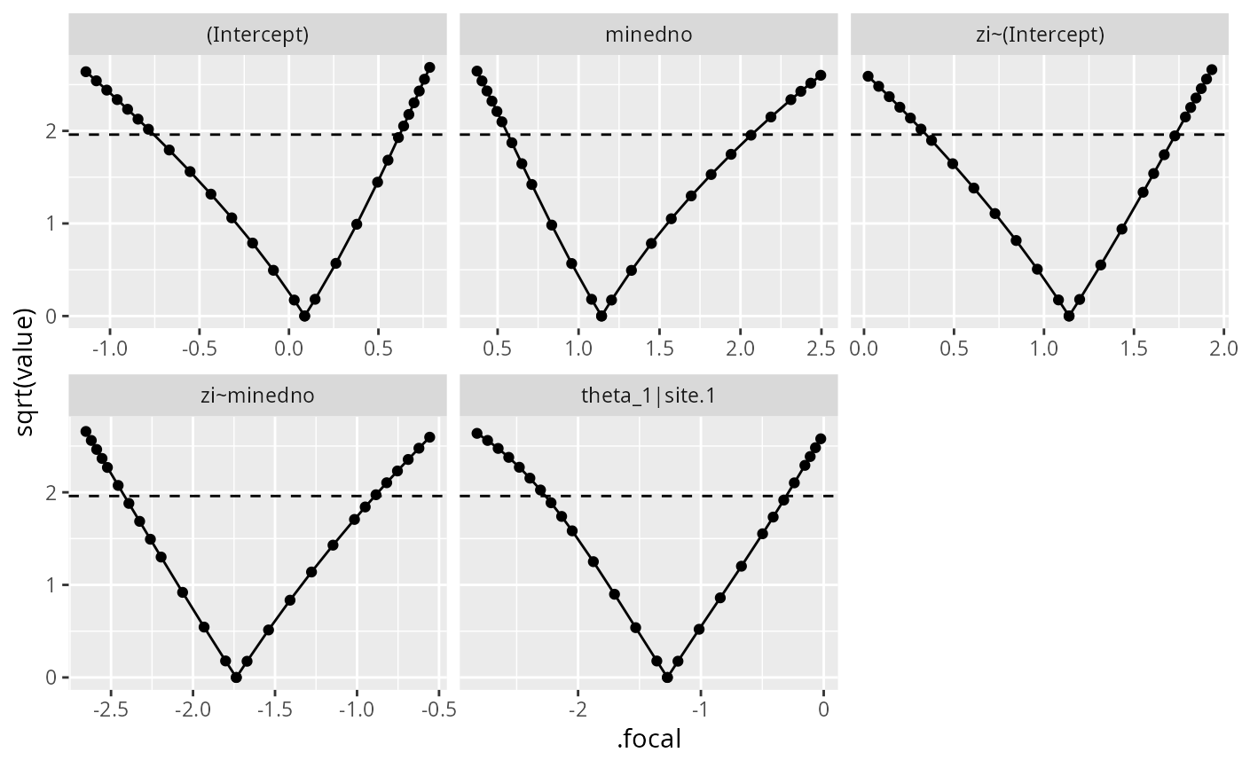
if (require("ggplot2")) {
    ggplot(salamander_prof1,aes(.focal,sqrt(value))) +
        geom_point() + geom_line()+
        facet_wrap(~.par,scale="free_x")+
    geom_hline(yintercept=1.96,linetype=2)
}
#> Loading required package: ggplot2

salamander_prof1 <- readRDS(system.file("example_files","salamander_prof1.rds",package="glmmTMB"))
confint(salamander_prof1)
#>                     2.5 %     97.5 %
#> (Intercept)    -0.4686460  0.4805030
#> minedno         0.6449938  1.7417972
#> zi~(Intercept)  0.6088771  1.5648495
#> zi~minedno     -2.2239195 -1.1665205
#> theta_1|site.1 -1.9452621 -0.5786442
confint(salamander_prof1,level=0.99)
#>                     0.5 %     99.5 %
#> (Intercept)    -0.6830922  0.5865649
#> minedno         0.6015779  1.9853898
#> zi~(Intercept)  0.4108581  1.6910201
#> zi~minedno     -2.3713049 -0.9600516
#> theta_1|site.1 -2.1810585 -0.3697326