Fit Models with TMB — glmmTMB • glmmTMB

Fit a generalized linear mixed model (GLMM) using Template Model Builder (TMB).

Usage

glmmTMB(
  formula,
  data = NULL,
  family = gaussian(),
  ziformula = ~0,
  dispformula = ~1,
  weights = NULL,
  offset = NULL,
  contrasts = NULL,
  na.action,
  se = TRUE,
  verbose = FALSE,
  doFit = TRUE,
  control = glmmTMBControl(),
  REML = FALSE,
  start = NULL,
  map = NULL,
  sparseX = NULL,
  priors = NULL,
  subset = NULL
)

Arguments

formula: combined fixed and random effects formula, following lme4 syntax.
data: data frame (tibbles are OK) containing model variables. Not required, but strongly recommended; if data is not specified, downstream methods such as prediction with new data (predict(fitted_model, newdata = ...)) will fail. If it is necessary to call glmmTMB with model variables taken from the environment rather than from a data frame, specifying data=NULL will suppress the warning message.
family: a family function, a character string naming a family function, or the result of a call to a family function (variance/link function) information. See family for a generic discussion of families or family_glmmTMB for details of glmmTMB-specific families.
ziformula: a one-sided (i.e., no response variable) formula for zero-inflation combining fixed and random effects: the default ~0 specifies no zero-inflation. Specifying ~. sets the zero-inflation formula identical to the right-hand side of formula (i.e., the conditional effects formula); terms can also be added or subtracted. When using ~. as the zero-inflation formula in models where the conditional effects formula contains an offset term, the offset term will automatically be dropped. The zero-inflation model uses a logit link.
dispformula: a one-sided formula for dispersion combining fixed and random effects: the default ~1 specifies the standard dispersion given any family. The argument is ignored for families that do not have a dispersion parameter. For an explanation of the dispersion parameter for each family, see sigma. The dispersion model uses a log link. In Gaussian mixed models, dispformula=~0 fixes the residual variance to be 0 (actually a small non-zero value), forcing variance into the random effects. The precise value can be controlled via control=glmmTMBControl(zero_dispval=...); the default value is sqrt(.Machine$double.eps).
weights: weights, as in glm. Not automatically scaled to have sum 1.
offset: offset for conditional model (only).
contrasts: an optional list, e.g., list(fac1="contr.sum"). See the contrasts.arg of model.matrix.default.
na.action: a function that specifies how to handle observations containing NAs. The default action (na.omit, inherited from the 'factory fresh' value of getOption("na.action")) strips any observations with any missing values in any variables. Using na.action = na.exclude will similarly drop observations with missing values while fitting the model, but will fill in NA values for the predicted and residual values for cases that were excluded during the fitting process because of missingness.
se: whether to return standard errors.
verbose: whether progress indication should be printed to the console.
doFit: whether to fit the full model, or (if FALSE) return the preprocessed data and parameter objects, without fitting the model.
control: control parameters, see glmmTMBControl.
REML: whether to use REML estimation rather than maximum likelihood.
start: starting values, expressed as a list with possible components beta, betazi, betadisp (fixed-effect parameters for conditional, zero-inflation, dispersion models); b, bzi, bdisp (conditional modes for conditional, zero-inflation, and dispersion models); theta, thetazi, thetadisp (random-effect parameters, on the standard deviation/Cholesky scale, for conditional, z-i, and disp models); psi (extra family parameters, e.g., shape for Tweedie models).
map: a list specifying which parameter values should be fixed to a constant value rather than estimated. map should be a named list containing factors corresponding to a subset of the internal parameter names (see start parameter). Distinct factor values are fitted as separate parameter values, NA values are held fixed: e.g., map=list(beta=factor(c(1,2,3,NA))) would fit the first three fixed-effect parameters of the conditional model and fix the fourth parameter to its starting value. In general, users will probably want to use start to specify non-default starting values for fixed parameters. See MakeADFun for more details.
sparseX: a named logical vector containing (possibly) elements named "cond", "zi", "disp" to indicate whether fixed-effect model matrices for particular model components should be generated as sparse matrices, e.g. c(cond=TRUE). Default is all FALSE
priors: a data frame of priors, in a similar format to that accepted by the brms package; see priors
subset: an optional vector specifying a subset of observations to be used in the fitting process (see model.frame)

Details

Binomial models with more than one trial (i.e., not binary/Bernoulli) can either be specified in the form prob ~ ..., weights = N, or in the more typical two-column matrix cbind(successes,failures)~... form.
Behavior of REML=TRUE for Gaussian responses matches lme4::lmer. It may also be useful in some cases with non-Gaussian responses (Millar 2011). Simulations should be done first to verify.
Because the df.residual method for glmmTMB currently counts the dispersion parameter, users should multiply this value by sqrt(nobs(fit) / (1+df.residual(fit))) when comparing with lm.
Although models can be fitted without specifying a data argument, its use is strongly recommended; drawing model components from the global environment, or using df$var notation within model formulae, can lead to confusing (and sometimes hard-to-detect) errors.
By default, vector-valued random effects are fitted with unstructured (general symmetric positive definite) variance-covariance matrices. Structured variance-covariance matrices can be specified in the form struc(terms|group), where struc is one of
- diag (diagonal, heterogeneous variance)
- ar1 (autoregressive order-1, homogeneous variance)
- hetar1 (autoregressive order-1, heterogeneous variance)
- cs (compound symmetric, heterogeneous variance)
- homcs (compound symmetric, homogeneous variance)
- ou (* Ornstein-Uhlenbeck, homogeneous variance)
- exp (* exponential autocorrelation)
- gau (* Gaussian autocorrelation)
- mat (* Matérn process correlation)
- toep (* Toeplitz, heterogeneous variance)
- homtoep (* Toeplitz, homogeneous variance)
- rr (reduced-rank/factor-analytic model)
- homdiag (diagonal, homogeneous variance)
- propto (* proportional to user-specified variance-covariance matrix)
- equalto (* equal to user-specified variance-covariance matrix)
Structures marked with * are experimental/untested. See vignette("covstruct", package = "glmmTMB") for more information.
For backward compatibility, the family argument can also be specified as a list comprising the name of the distribution and the link function (e.g. list(family="binomial", link="logit")). However, this alternative is now deprecated; it produces a warning and will be removed at some point in the future. Furthermore, certain capabilities such as Pearson residuals or predictions on the data scale will only be possible if components such as variance and linkfun are present, see family.
Smooths taken from the mgcv package can be included in glmmTMB formulas using s; these terms will appear as additional components in both the fixed and the random-effects terms. This functionality is experimental for now. We recommend using REML=TRUE. See s for details of specifying smooths (and smooth2random and the appendix of Wood (2004) for technical details).

Note

For more information about the glmmTMB package, see Brooks et al. (2017) and the vignette(package="glmmTMB") collection. For the underlying TMB package that performs the model estimation, see Kristensen et al. (2016).

References

Brooks, M. E., Kristensen, K., van Benthem, K. J., Magnusson, A., Berg, C. W., Nielsen, A., Skaug, H. J., Mächler, M. and Bolker, B. M. (2017). glmmTMB balances speed and flexibility among packages for zero-inflated generalized linear mixed modeling. The R Journal, 9(2), 378–400.

Kristensen, K., Nielsen, A., Berg, C. W., Skaug, H. and Bell, B. (2016). TMB: Automatic differentiation and Laplace approximation. Journal of Statistical Software, 70, 1–21.

Millar, R. B. (2011). Maximum Likelihood Estimation and Inference: With Examples in R, SAS and ADMB. Wiley, New York. Wood, S. N. (2004) Stable and Efficient Multiple Smoothing Parameter Estimation for Generalized Additive Models. Journal of the American Statistical Association 99(467): 673–86. doi:10.1198/016214504000000980

Examples

# \donttest{
(m1 <- glmmTMB(count ~ mined + (1|site),
  zi=~mined,
  family=poisson, data=Salamanders))
#> Formula:          count ~ mined + (1 | site)
#> Zero inflation:         ~mined
#> Data: Salamanders
#>       AIC       BIC    logLik -2*log(L)  df.resid 
#> 1908.4695 1930.8080 -949.2348 1898.4695       639 
#> Random-effects (co)variances:
#> 
#> Conditional model:
#>  Groups Name        Std.Dev.
#>  site   (Intercept) 0.28    
#> 
#> Number of obs: 644 / Conditional model: site, 23
#> 
#> Fixed Effects:
#> 
#> Conditional model:
#> (Intercept)      minedno  
#>      0.0879       1.1419  
#> 
#> Zero-inflation model:
#> (Intercept)      minedno  
#>       1.139       -1.736  
summary(m1)
#>  Family: poisson  ( log )
#> Formula:          count ~ mined + (1 | site)
#> Zero inflation:         ~mined
#> Data: Salamanders
#> 
#>       AIC       BIC    logLik -2*log(L)  df.resid 
#>    1908.5    1930.8    -949.2    1898.5       639 
#> 
#> Random effects:
#> 
#> Conditional model:
#>  Groups Name        Variance Std.Dev.
#>  site   (Intercept) 0.07843  0.28    
#> Number of obs: 644, groups:  site, 23
#> 
#> Conditional model:
#>             Estimate Std. Error z value Pr(>|z|)    
#> (Intercept)   0.0879     0.2329   0.377    0.706    
#> minedno       1.1419     0.2462   4.639  3.5e-06 ***
#> ---
#> Signif. codes:  0 ‘***’ 0.001 ‘**’ 0.01 ‘*’ 0.05 ‘.’ 0.1 ‘ ’ 1
#> 
#> Zero-inflation model:
#>             Estimate Std. Error z value Pr(>|z|)    
#> (Intercept)   1.1393     0.2351   4.846 1.26e-06 ***
#> minedno      -1.7361     0.2620  -6.626 3.44e-11 ***
#> ---
#> Signif. codes:  0 ‘***’ 0.001 ‘**’ 0.01 ‘*’ 0.05 ‘.’ 0.1 ‘ ’ 1
##' ## Zero-inflated negative binomial model
(m2 <- glmmTMB(count ~ spp + mined + (1|site),
  zi=~spp + mined,
  family=nbinom2, data=Salamanders))
#> Formula:          count ~ spp + mined + (1 | site)
#> Zero inflation:         ~spp + mined
#> Data: Salamanders
#>       AIC       BIC    logLik -2*log(L)  df.resid 
#> 1670.2990 1750.7176 -817.1495 1634.2990       626 
#> Random-effects (co)variances:
#> 
#> Conditional model:
#>  Groups Name        Std.Dev.
#>  site   (Intercept) 0.3799  
#> 
#> Number of obs: 644 / Conditional model: site, 23
#> 
#> Dispersion parameter for nbinom2 family (): 1.51 
#> 
#> Fixed Effects:
#> 
#> Conditional model:
#> (Intercept)        sppPR        sppDM      sppEC-A      sppEC-L     sppDES-L  
#>     -0.6104      -0.9637       0.1707      -0.3871       0.4879       0.5895  
#>       sppDF      minedno  
#>     -0.1133       1.4294  
#> 
#> Zero-inflation model:
#> (Intercept)        sppPR        sppDM      sppEC-A      sppEC-L     sppDES-L  
#>      0.9100       1.1614      -0.9393       1.0424      -0.5623      -0.8930  
#>       sppDF      minedno  
#>     -2.5398      -2.5630  

## Hurdle Poisson model
(m3 <- glmmTMB(count ~ spp + mined + (1|site),
  zi=~spp + mined,
  family=truncated_poisson, data=Salamanders))
#> Formula:          count ~ spp + mined + (1 | site)
#> Zero inflation:         ~spp + mined
#> Data: Salamanders
#>       AIC       BIC    logLik -2*log(L)  df.resid 
#> 1790.1669 1866.1177 -878.0834 1756.1669       627 
#> Random-effects (co)variances:
#> 
#> Conditional model:
#>  Groups Name        Std.Dev.
#>  site   (Intercept) 0.2306  
#> 
#> Number of obs: 644 / Conditional model: site, 23
#> 
#> Fixed Effects:
#> 
#> Conditional model:
#> (Intercept)        sppPR        sppDM      sppEC-A      sppEC-L     sppDES-L  
#>    -0.06702     -0.52093      0.22458     -0.19548      0.64672      0.60514  
#>       sppDF      minedno  
#>     0.04602      1.01447  
#> 
#> Zero-inflation model:
#> (Intercept)        sppPR        sppDM      sppEC-A      sppEC-L     sppDES-L  
#>      1.7556       1.6785      -0.4269       1.1046      -0.4269      -0.6716  
#>       sppDF      minedno  
#>     -0.4269      -2.4038  

## Binomial model
data(cbpp, package="lme4")
(bovine <- glmmTMB(cbind(incidence, size-incidence) ~ period + (1|herd),
  family=binomial, data=cbpp))
#> Formula:          cbind(incidence, size - incidence) ~ period + (1 | herd)
#> Data: cbpp
#>       AIC       BIC    logLik -2*log(L)  df.resid 
#> 194.05256 204.17932 -92.02628 184.05256        51 
#> Random-effects (co)variances:
#> 
#> Conditional model:
#>  Groups Name        Std.Dev.
#>  herd   (Intercept) 0.6423  
#> 
#> Number of obs: 56 / Conditional model: herd, 15
#> 
#> Fixed Effects:
#> 
#> Conditional model:
#> (Intercept)      period2      period3      period4  
#>     -1.3985      -0.9923      -1.1287      -1.5803  

## Dispersion model
sim1 <- function(nfac=40, nt=100, facsd=0.1, tsd=0.15, mu=0, residsd=1)
{
  dat <- expand.grid(fac=factor(letters[1:nfac]), t=1:nt)
  n <- nrow(dat)
  dat$REfac <- rnorm(nfac, sd=facsd)[dat$fac]
  dat$REt <- rnorm(nt, sd=tsd)[dat$t]
  dat$x <- rnorm(n, mean=mu, sd=residsd) + dat$REfac + dat$REt
  dat
}
set.seed(101)
d1 <- sim1(mu=100, residsd=10)
d2 <- sim1(mu=200, residsd=5)
d1$sd <- "ten"
d2$sd <- "five"
dat <- rbind(d1, d2)
m0 <- glmmTMB(x ~ sd + (1|t), dispformula=~sd, data=dat)
fixef(m0)$disp
#> (Intercept)       sdten 
#>   1.6014350   0.6932378 
c(log(5), log(10)-log(5)) # expected dispersion model coefficients
#> [1] 1.6094379 0.6931472


## Using 'map' to fix random-effects SD to 10
m1_map <- update(m1, map=list(theta=factor(NA)),
                 start=list(theta=log(10)))
VarCorr(m1_map)
#> 
#> Conditional model:
#>  Groups Name        Std.Dev.
#>  site   (Intercept) 10      

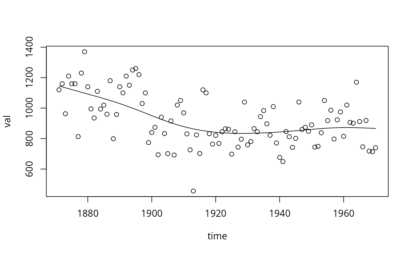
## smooth terms
data("Nile")
ndat <- data.frame(time = c(time(Nile)), val = c(Nile))
sm1 <- glmmTMB(val ~ s(time), data = ndat,
               REML = TRUE, start = list(theta = 5))
plot(val ~ time, data = ndat)
lines(ndat$time, predict(sm1))


## reduced-rank model
m1_rr <- glmmTMB(abund ~ Species + rr(Species + 0|id, d = 1),
                              data = spider_long)
# }