stat_quadrant_counts() counts the number of observations in each
quadrant of a plot panel. By default it adds a text label to the far corner
of each quadrant. It can also be used to obtain the total number of
observations in each of two pairs of quadrants or in the whole panel.
Grouping is ignored, so en every case a single count is computed for each
quadrant in a plot panel.
stat_quadrant_counts(
  mapping = NULL,
  data = NULL,
  geom = "text_npc",
  position = "identity",
  quadrants = NULL,
  pool.along = c("none", "x", "y", "xy"),
  xintercept = 0,
  yintercept = 0,
  label.x = NULL,
  label.y = NULL,
  digits = 2,
  na.rm = FALSE,
  show.legend = FALSE,
  inherit.aes = TRUE,
  ...
)
Arguments
- mapping
The aesthetic mapping, usually constructed with
aesoraes_. Only needs to be set at the layer level if you are overriding the plot defaults.- data
A layer specific dataset - only needed if you want to override the plot defaults.
- geom
The geometric object to use display the data
- position
The position adjustment to use on this layer
- quadrants
integer vector indicating which quadrants are of interest, with a
OLindicating the whole plot.- pool.along
character, one of
"none","x"or"y", indicating which quadrants to pool to calculate counts by pair of quadrants.- xintercept, yintercept
numeric the coordinates of the origin of the quadrants.
- label.x, label.y
numericCoordinates (in npc units) to be used for absolute positioning of the labels.- digits
integer Number of digits for fraction and percent labels.
- na.rm
a logical indicating whether
NAvalues should be stripped before the computation proceeds.- show.legend
logical. Should this layer be included in the legends?
NA, the default, includes if any aesthetics are mapped.FALSEnever includes, andTRUEalways includes.- inherit.aes
If
FALSE, overrides the default aesthetics, rather than combining with them. This is most useful for helper functions that define both data and aesthetics and should not inherit behaviour from the default plot specification, e.g.,borders.- ...
other arguments passed on to
layer. This can include aesthetics whose values you want to set, not map. Seelayerfor more details.
Value
A plot layer instance. Using as output data the counts of
observations per plot quadrant.
Details
This statistic can be used to automatically count observations in
each of the four quadrants of a plot, and by default add these counts as
text labels. Values exactly equal to xintercept or
yintercept are counted together with those larger than the
intercepts. An argument value of zero, passed to formal parameter
quadrants is interpreted as a request for the count of all
observations in each plot panel.
The default origin of quadrants is at xintercept = 0,
yintercept = 0. Also by default, counts are computed for all
quadrants within the x and y scale limits, but ignoring any
marginal scale expansion. The default positions of the labels is in the
farthest corner or edge of each quadrant using npc coordinates.
Consequently, when using facets even with free limits for x and
y axes, the location of the labels is consistent across panels. This
is achieved by use of geom = "text_npc" or geom =
"label_npc". To pass the positions in native data units, pass geom =
"text" explicitly as argument.
Computed variables
Data frame with one to four rows, one for each
quadrant for which counts are counted in data.
- quadrant
integer, one of 0:4
- x
x value of label position in data units
- y
y value of label position in data units
- npcx
x value of label position in npc units
- npcy
y value of label position in npc units
- count
number of observations in the quadrant(s)
- total
number of onservations in data
- count.label
number of observations as character
- pc.label
percent of observations as character
- fr.label
fraction of observations as character
.
As shown in one example below geom_debug can be
used to print the computed values returned by any statistic. The output
shown includes also values mapped to aesthetics, like label in the
example.
See also
Other Functions for quadrant and volcano plots:
geom_quadrant_lines(),
stat_panel_counts()
Examples
# generate artificial data
set.seed(4321)
x <- -50:50
y <- rnorm(length(x), mean = 0)
my.data <- data.frame(x, y)
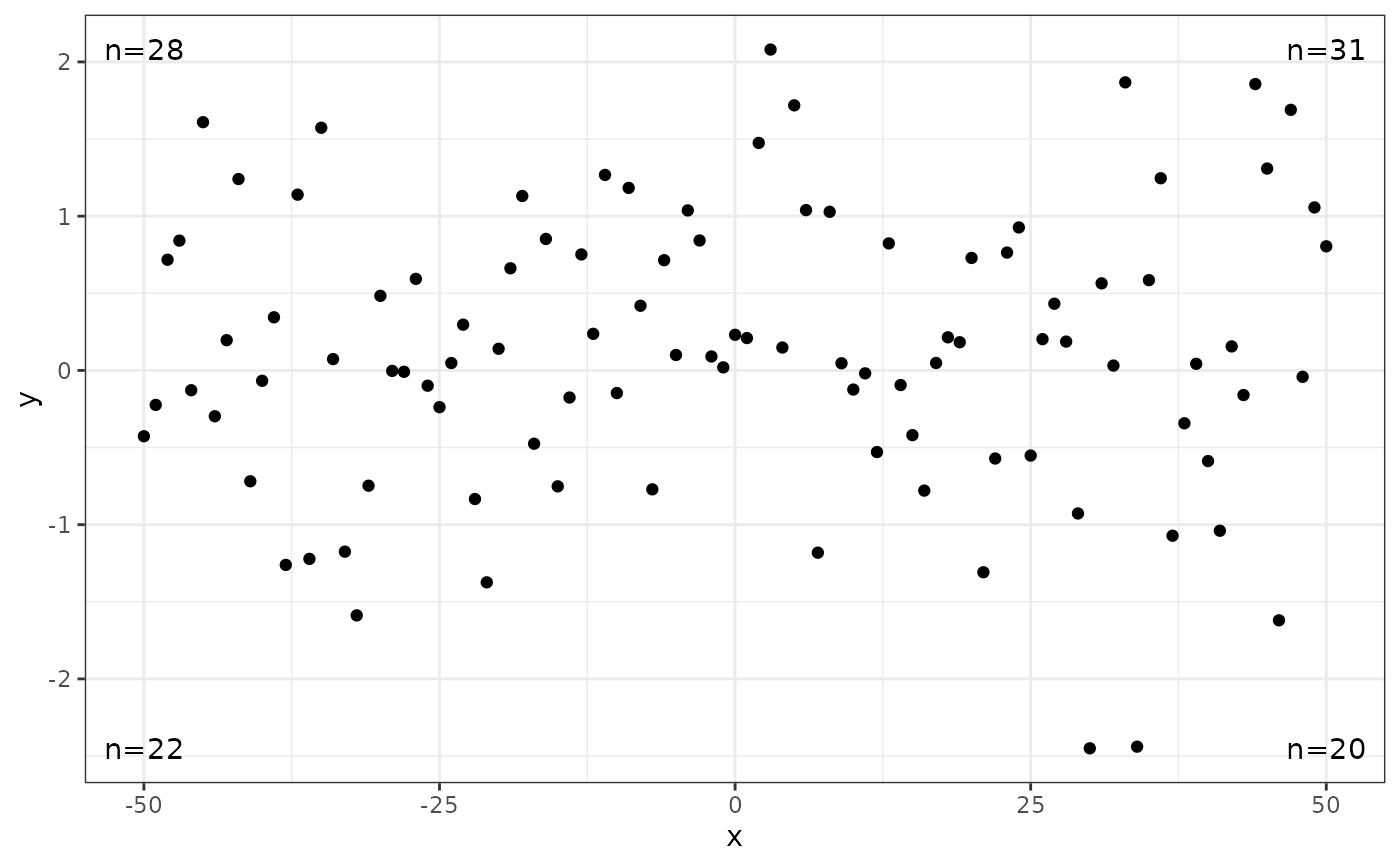
# using automatically generated text labels, default origin at (0, 0)
ggplot(my.data, aes(x, y)) +
geom_point() +
geom_quadrant_lines() +
stat_quadrant_counts()
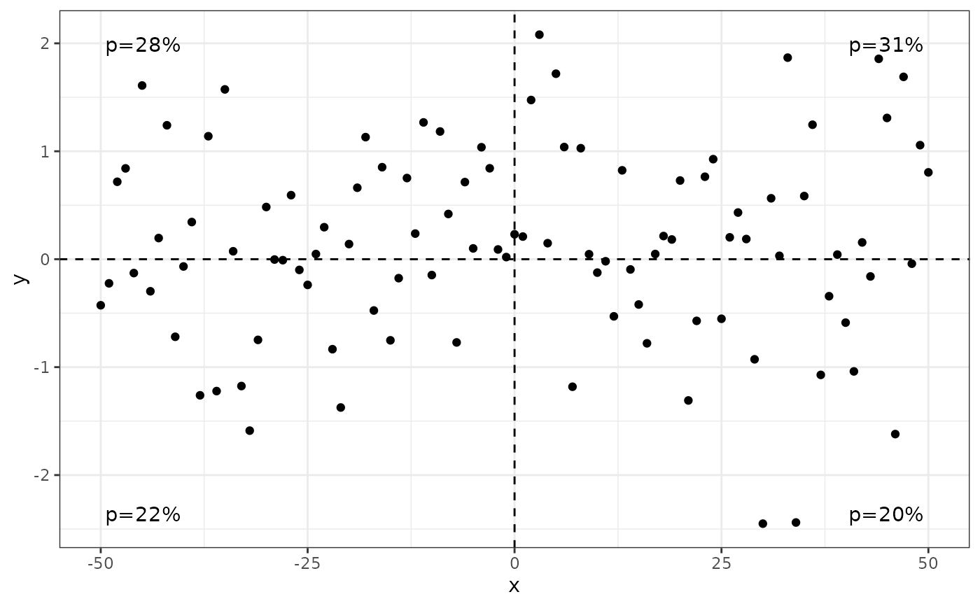
 ggplot(my.data, aes(x, y)) +
geom_point() +
geom_quadrant_lines() +
stat_quadrant_counts(aes(label = after_stat(pc.label)))
ggplot(my.data, aes(x, y)) +
geom_point() +
geom_quadrant_lines() +
stat_quadrant_counts(aes(label = after_stat(pc.label)))
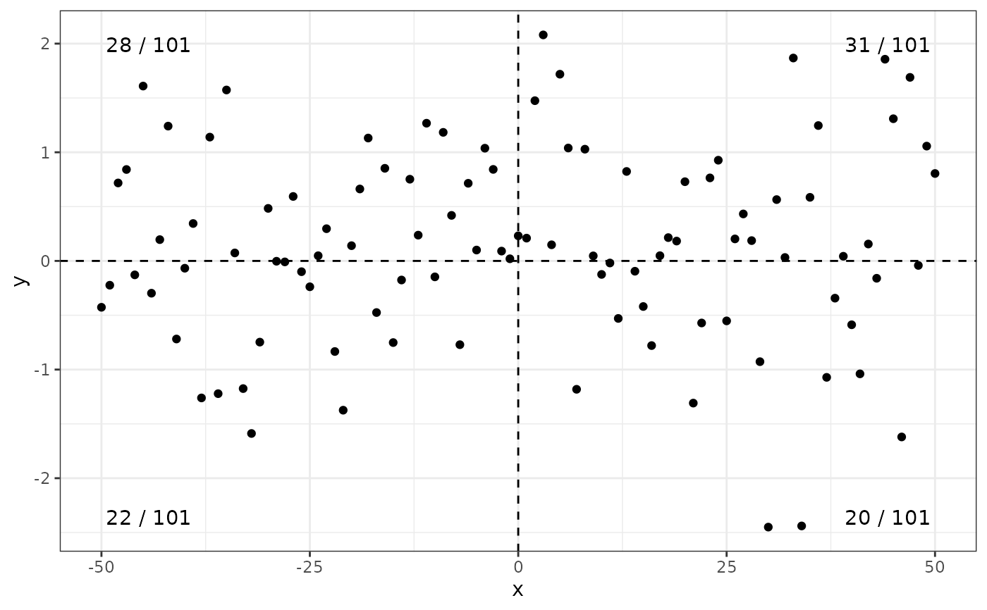
 ggplot(my.data, aes(x, y)) +
geom_point() +
geom_quadrant_lines() +
stat_quadrant_counts(aes(label = after_stat(fr.label)))
ggplot(my.data, aes(x, y)) +
geom_point() +
geom_quadrant_lines() +
stat_quadrant_counts(aes(label = after_stat(fr.label)))
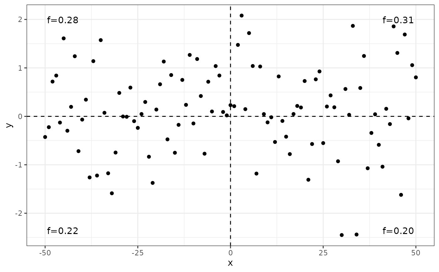
 ggplot(my.data, aes(x, y)) +
geom_point() +
geom_quadrant_lines() +
stat_quadrant_counts(aes(label = after_stat(dec.label)))
ggplot(my.data, aes(x, y)) +
geom_point() +
geom_quadrant_lines() +
stat_quadrant_counts(aes(label = after_stat(dec.label)))
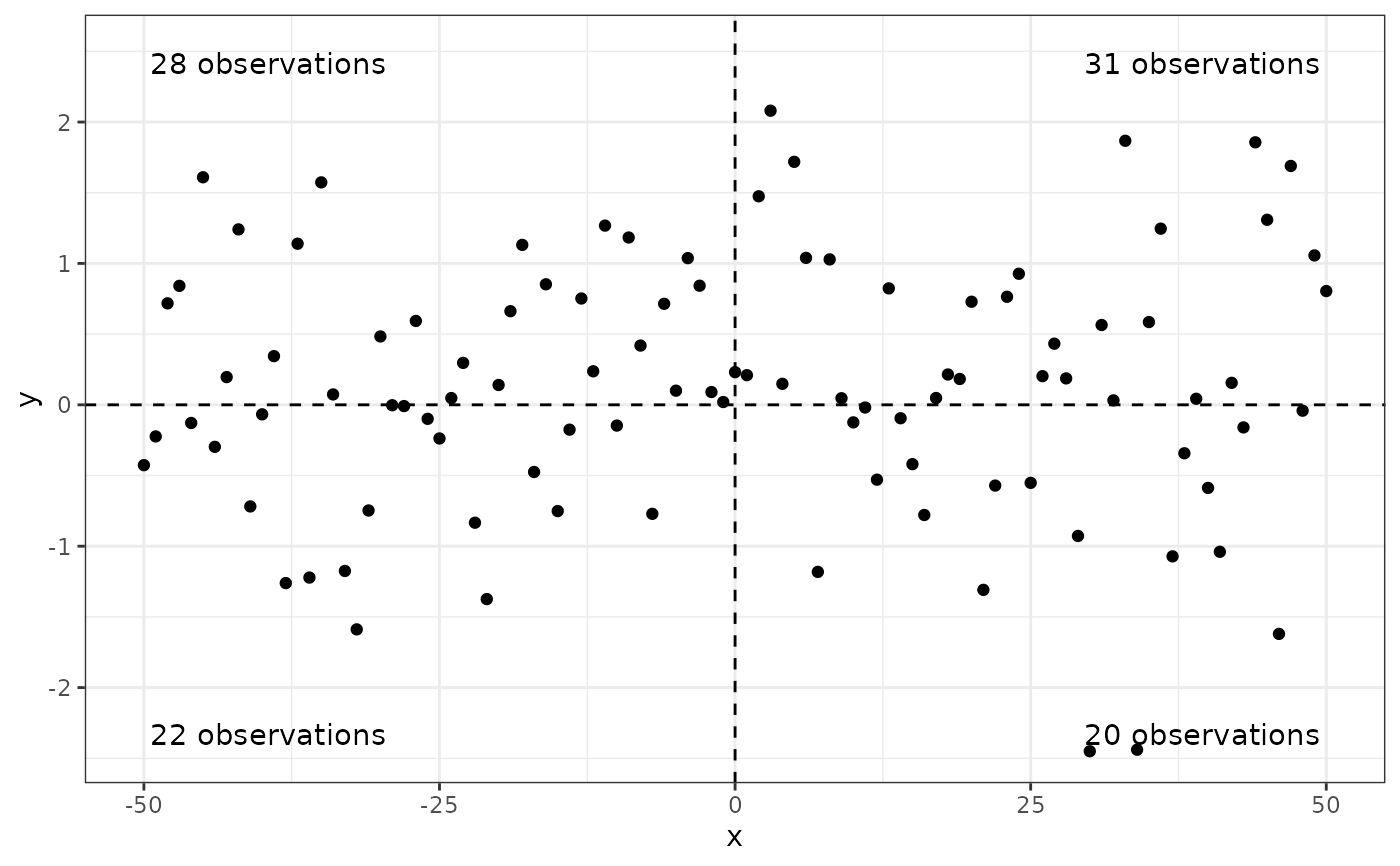
 ggplot(my.data, aes(x, y)) +
geom_point() +
geom_quadrant_lines() +
stat_quadrant_counts(aes(label = sprintf("%i observations", after_stat(count)))) +
scale_y_continuous(expand = expansion(c(0.05, 0.15))) # reserve space
ggplot(my.data, aes(x, y)) +
geom_point() +
geom_quadrant_lines() +
stat_quadrant_counts(aes(label = sprintf("%i observations", after_stat(count)))) +
scale_y_continuous(expand = expansion(c(0.05, 0.15))) # reserve space
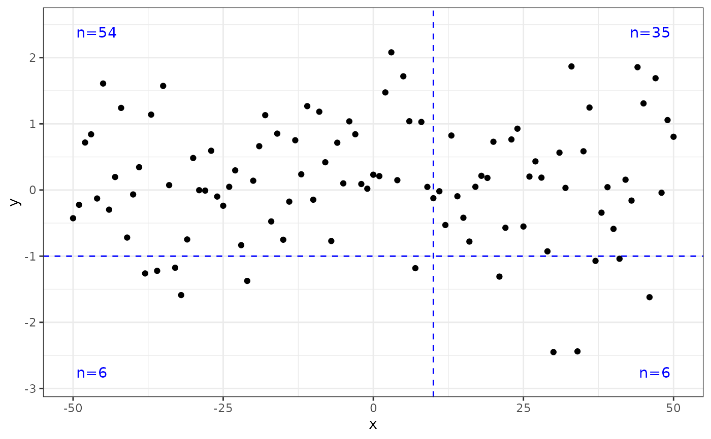
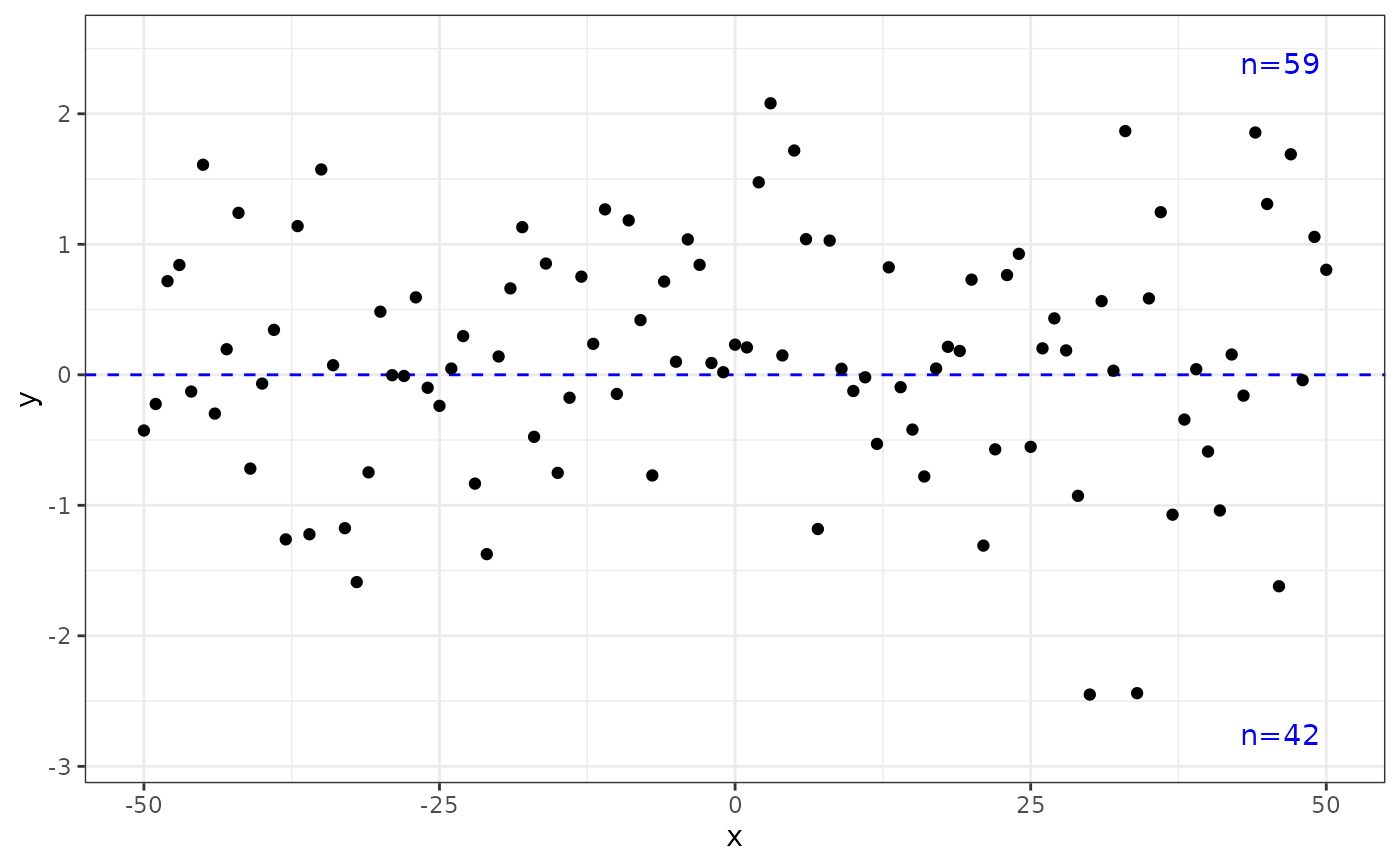
 # user specified origin
ggplot(my.data, aes(x, y)) +
geom_quadrant_lines(colour = "blue", xintercept = 10, yintercept = -1) +
stat_quadrant_counts(colour = "blue", xintercept = 10, yintercept = -1) +
geom_point() +
scale_y_continuous(expand = expansion(mult = 0.15))
# user specified origin
ggplot(my.data, aes(x, y)) +
geom_quadrant_lines(colour = "blue", xintercept = 10, yintercept = -1) +
stat_quadrant_counts(colour = "blue", xintercept = 10, yintercept = -1) +
geom_point() +
scale_y_continuous(expand = expansion(mult = 0.15))
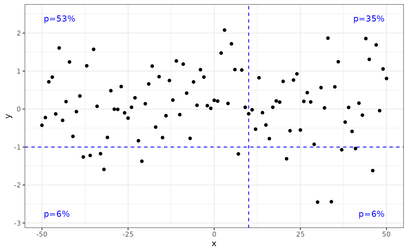
 ggplot(my.data, aes(x, y)) +
geom_quadrant_lines(colour = "blue", xintercept = 10, yintercept = -1) +
stat_quadrant_counts(aes(label = after_stat(pc.label)),
colour = "blue", xintercept = 10, yintercept = -1) +
geom_point() +
scale_y_continuous(expand = expansion(mult = 0.15))
ggplot(my.data, aes(x, y)) +
geom_quadrant_lines(colour = "blue", xintercept = 10, yintercept = -1) +
stat_quadrant_counts(aes(label = after_stat(pc.label)),
colour = "blue", xintercept = 10, yintercept = -1) +
geom_point() +
scale_y_continuous(expand = expansion(mult = 0.15))
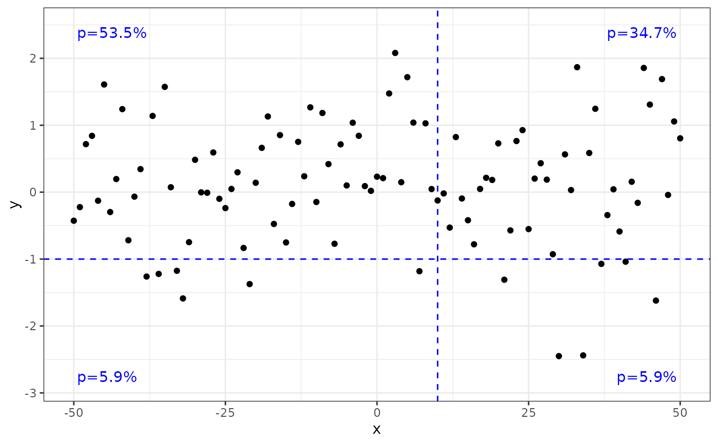
 # more digits in labels
ggplot(my.data, aes(x, y)) +
geom_quadrant_lines(colour = "blue", xintercept = 10, yintercept = -1) +
stat_quadrant_counts(aes(label = after_stat(pc.label)), digits = 3,
colour = "blue", xintercept = 10, yintercept = -1) +
geom_point() +
scale_y_continuous(expand = expansion(mult = 0.15))
# more digits in labels
ggplot(my.data, aes(x, y)) +
geom_quadrant_lines(colour = "blue", xintercept = 10, yintercept = -1) +
stat_quadrant_counts(aes(label = after_stat(pc.label)), digits = 3,
colour = "blue", xintercept = 10, yintercept = -1) +
geom_point() +
scale_y_continuous(expand = expansion(mult = 0.15))
 ggplot(my.data, aes(x, y)) +
geom_quadrant_lines(colour = "blue", xintercept = 10, yintercept = -1) +
stat_quadrant_counts(aes(label = after_stat(fr.label)),
colour = "blue", xintercept = 10, yintercept = -1) +
geom_point() +
scale_y_continuous(expand = expansion(mult = 0.15))
ggplot(my.data, aes(x, y)) +
geom_quadrant_lines(colour = "blue", xintercept = 10, yintercept = -1) +
stat_quadrant_counts(aes(label = after_stat(fr.label)),
colour = "blue", xintercept = 10, yintercept = -1) +
geom_point() +
scale_y_continuous(expand = expansion(mult = 0.15))
 # grouped quadrants
ggplot(my.data, aes(x, y)) +
geom_quadrant_lines(colour = "blue",
pool.along = "x") +
stat_quadrant_counts(colour = "blue", label.x = "right",
pool.along = "x") +
geom_point() +
scale_y_continuous(expand = expansion(mult = 0.15))
# grouped quadrants
ggplot(my.data, aes(x, y)) +
geom_quadrant_lines(colour = "blue",
pool.along = "x") +
stat_quadrant_counts(colour = "blue", label.x = "right",
pool.along = "x") +
geom_point() +
scale_y_continuous(expand = expansion(mult = 0.15))
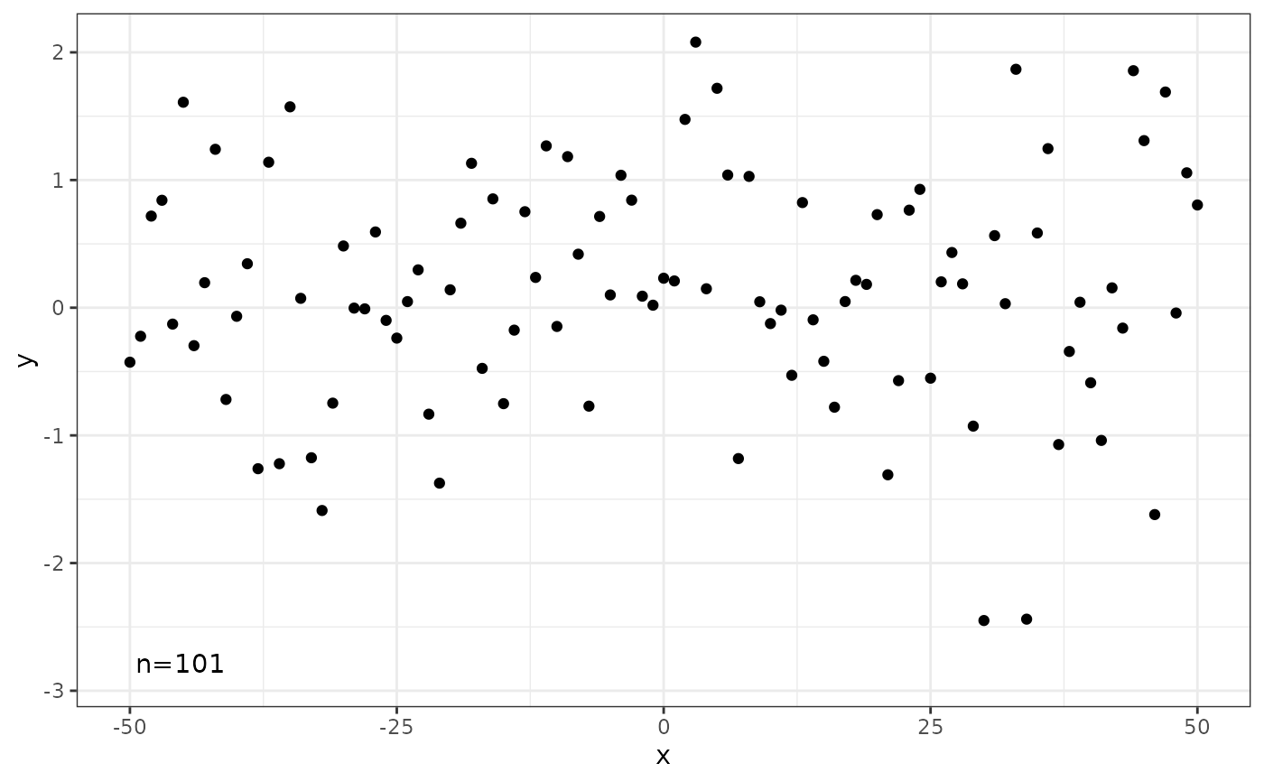
 # whole panel
ggplot(my.data, aes(x, y)) +
geom_point() +
stat_quadrant_counts(quadrants = 0, label.x = "left", label.y = "bottom") +
scale_y_continuous(expand = expansion(mult = c(0.15, 0.05)))
# whole panel
ggplot(my.data, aes(x, y)) +
geom_point() +
stat_quadrant_counts(quadrants = 0, label.x = "left", label.y = "bottom") +
scale_y_continuous(expand = expansion(mult = c(0.15, 0.05)))
 # use a different geometry
ggplot(my.data, aes(x, y)) +
geom_point() +
stat_quadrant_counts(geom = "text") # use geom_text()
# use a different geometry
ggplot(my.data, aes(x, y)) +
geom_point() +
stat_quadrant_counts(geom = "text") # use geom_text()
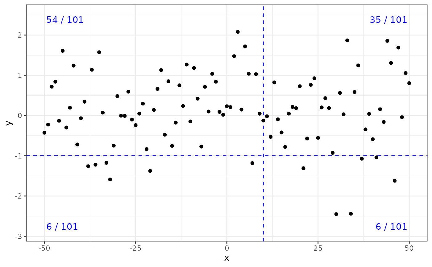
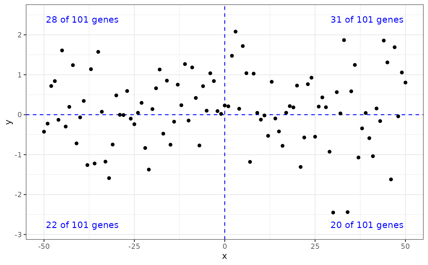
 # Numeric values can be used to build labels with alternative formats
# Here with sprintf(), but paste() and format() also work.
ggplot(my.data, aes(x, y)) +
geom_quadrant_lines(colour = "blue") +
stat_quadrant_counts(aes(label = sprintf("%i of %i genes",
after_stat(count), after_stat(total))),
colour = "blue") +
geom_point() +
scale_y_continuous(expand = expansion(mult = 0.15))
# Numeric values can be used to build labels with alternative formats
# Here with sprintf(), but paste() and format() also work.
ggplot(my.data, aes(x, y)) +
geom_quadrant_lines(colour = "blue") +
stat_quadrant_counts(aes(label = sprintf("%i of %i genes",
after_stat(count), after_stat(total))),
colour = "blue") +
geom_point() +
scale_y_continuous(expand = expansion(mult = 0.15))
 # We use geom_debug() to see the computed values
gginnards.installed <- requireNamespace("gginnards", quietly = TRUE)
if (gginnards.installed) {
library(gginnards)
ggplot(my.data, aes(x, y)) +
geom_point() +
stat_quadrant_counts(geom = "debug")
ggplot(my.data, aes(x, y)) +
geom_point() +
stat_quadrant_counts(geom = "debug", xintercept = 50)
}
# We use geom_debug() to see the computed values
gginnards.installed <- requireNamespace("gginnards", quietly = TRUE)
if (gginnards.installed) {
library(gginnards)
ggplot(my.data, aes(x, y)) +
geom_point() +
stat_quadrant_counts(geom = "debug")
ggplot(my.data, aes(x, y)) +
geom_point() +
stat_quadrant_counts(geom = "debug", xintercept = 50)
}
 #> [1] "PANEL 1; group(s) NULL; 'draw_function()' input 'data' (head):"
#> npcx npcy label PANEL x y quadrant count total count.label pc.label
#> 1 0.95 0.95 n=1 1 50 2.080248 1 1 101 n=1 p=1%
#> 2 0.05 0.05 n=42 1 -50 -2.450016 3 42 101 n=42 p=42%
#> 3 0.05 0.95 n=58 1 -50 2.080248 4 58 101 n=58 p=57%
#> 4 0.95 0.05 n=0 1 50 -2.450016 2 0 101 n=0 p=0%
#> dec.label fr.label xintercept yintercept
#> 1 f=0.01 1 / 101 50 0
#> 2 f=0.42 42 / 101 50 0
#> 3 f=0.57 58 / 101 50 0
#> 4 f=0.00 0 / 101 50 0
#> [1] "PANEL 1; group(s) NULL; 'draw_function()' input 'data' (head):"
#> npcx npcy label PANEL x y quadrant count total count.label pc.label
#> 1 0.95 0.95 n=1 1 50 2.080248 1 1 101 n=1 p=1%
#> 2 0.05 0.05 n=42 1 -50 -2.450016 3 42 101 n=42 p=42%
#> 3 0.05 0.95 n=58 1 -50 2.080248 4 58 101 n=58 p=57%
#> 4 0.95 0.05 n=0 1 50 -2.450016 2 0 101 n=0 p=0%
#> dec.label fr.label xintercept yintercept
#> 1 f=0.01 1 / 101 50 0
#> 2 f=0.42 42 / 101 50 0
#> 3 f=0.57 58 / 101 50 0
#> 4 f=0.00 0 / 101 50 0