stat_panel_counts() counts the number of observations in each panel.
stat_group_counts() counts the number of observations in each group.
By default they add one or more text labels to the top right corner of each
panel. Grouping is ignored by stat_panel_counts(). If no grouping
exists, the two statistics behave similarly.
stat_panel_counts(
  mapping = NULL,
  data = NULL,
  geom = "text_npc",
  position = "identity",
  label.x = "right",
  label.y = "top",
  na.rm = FALSE,
  show.legend = FALSE,
  inherit.aes = TRUE,
  ...
)

stat_group_counts(
  mapping = NULL,
  data = NULL,
  geom = "text_npc",
  position = "identity",
  label.x = "right",
  label.y = "top",
  hstep = 0,
  vstep = NULL,
  digits = 2,
  na.rm = FALSE,
  show.legend = FALSE,
  inherit.aes = TRUE,
  ...
)
Arguments
- mapping
The aesthetic mapping, usually constructed with
aesoraes_. Only needs to be set at the layer level if you are overriding the plot defaults.- data
A layer specific dataset. Rarely used, as you will not want to override the plot defaults.
- geom
The geometric object to use display the data
- position
The position adjustment to use on this layer
- label.x, label.y
numericCoordinates (in npc units) to be used for absolute positioning of the labels.- na.rm
a logical indicating whether
NAvalues should be stripped before the computation proceeds.- show.legend
logical. Should this layer be included in the legends?
NA, the default, includes it if any aesthetics are mapped.FALSEnever includes, andTRUEalways includes.- inherit.aes
If
FALSE, overrides the default aesthetics, rather than combining with them. This is most useful for helper functions that define both data and aesthetics and should not inherit behaviour from the default plot specification, e.g.,borders.- ...
other arguments passed on to
layer. This can include aesthetics whose values you want to set, not map. Seelayerfor more details.- hstep, vstep
numeric in npc units, the horizontal and vertical step used between labels for different groups.
- digits
integer Number of digits for fraction and percent labels.
Value
A plot layer instance. Using as output data the counts of
observations in each plot panel or per group in each plot panel.
Details
These statistics can be used to automatically count observations in
each panel of a plot, and by default add these counts as text labels. These
statistics, unlike stat_quadrant_counts() requires only one of
x or y aesthetics and can be used together with statistics
that have the same requirement, like stat_density().
The default position of the label is in the top right corner. When using
facets even with free limits for x and y axes, the location
of the labels is consistent across panels. This is achieved by use of
geom = "text_npc" or geom = "label_npc". To pass the
positions in native data units to label.x and label.y, pass
also explicitly geom = "text", geom = "label" or some other
geometry that use the x and/or y aesthetics. A vector with
the same length as the number of panels in the figure can be used if
needed.
Note
If a factor is mapped to x or to y aesthetics each level
of the factor constitutes a group, in this case the default positioning and
geom using NPC pseudo aesthetics will have to be overriden by passing
geom = "text" and data coordinates used. The default for factors
may change in the future.
Computed variables
Data frame with one or more rows, one for each
group of observations for which counts are counted in data.
- x,npcx
x value of label position in data- or npc units, respectively
- y,npcy
y value of label position in data- or npc units, respectively
- count
number of observations as an integer
- count.label
number of observations as character
As shown in one example below geom_debug can be
used to print the computed values returned by any statistic. The output
shown includes also values mapped to aesthetics, like label in the
example. x and y are included in the output only if mapped.
See also
Other Functions for quadrant and volcano plots:
geom_quadrant_lines(),
stat_quadrant_counts()
Examples
# generate artificial data with numeric x and y
set.seed(67821)
x <- 1:100
y <- rnorm(length(x), mean = 10)
group <- factor(rep(c("A", "B"), times = 50))
my.data <- data.frame(x, y, group)
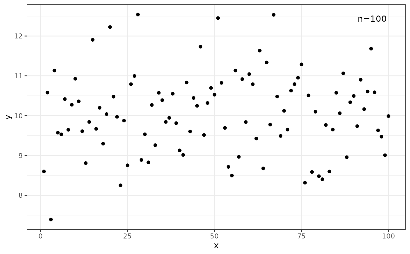
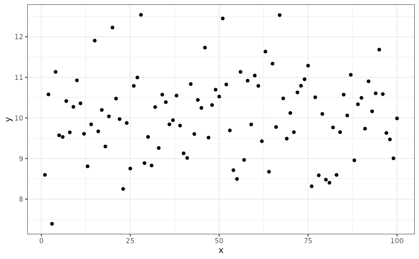
# using automatically generated text labels
ggplot(my.data, aes(x, y)) +
geom_point() +
stat_panel_counts()
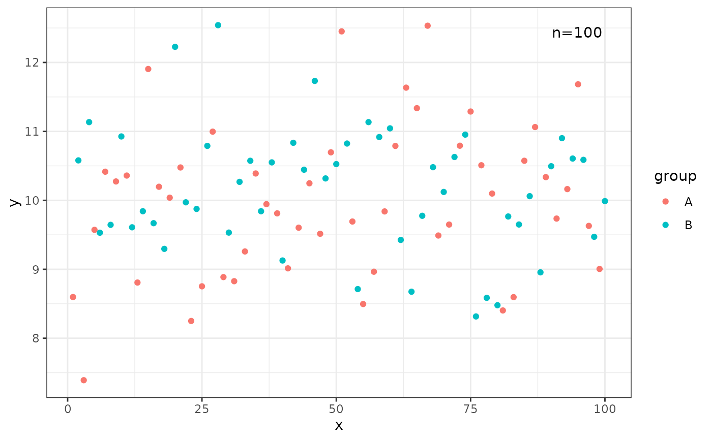
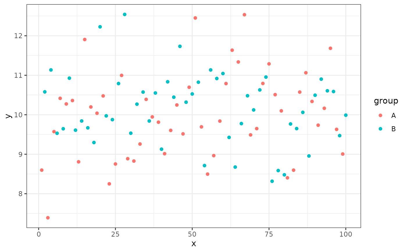
 ggplot(my.data, aes(x, y, colour = group)) +
geom_point() +
stat_panel_counts()
ggplot(my.data, aes(x, y, colour = group)) +
geom_point() +
stat_panel_counts()
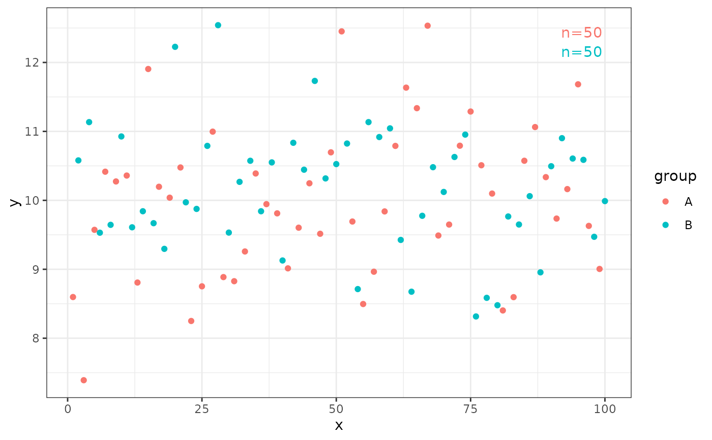
 ggplot(my.data, aes(x, y, colour = group)) +
geom_point() +
stat_group_counts()
ggplot(my.data, aes(x, y, colour = group)) +
geom_point() +
stat_group_counts()
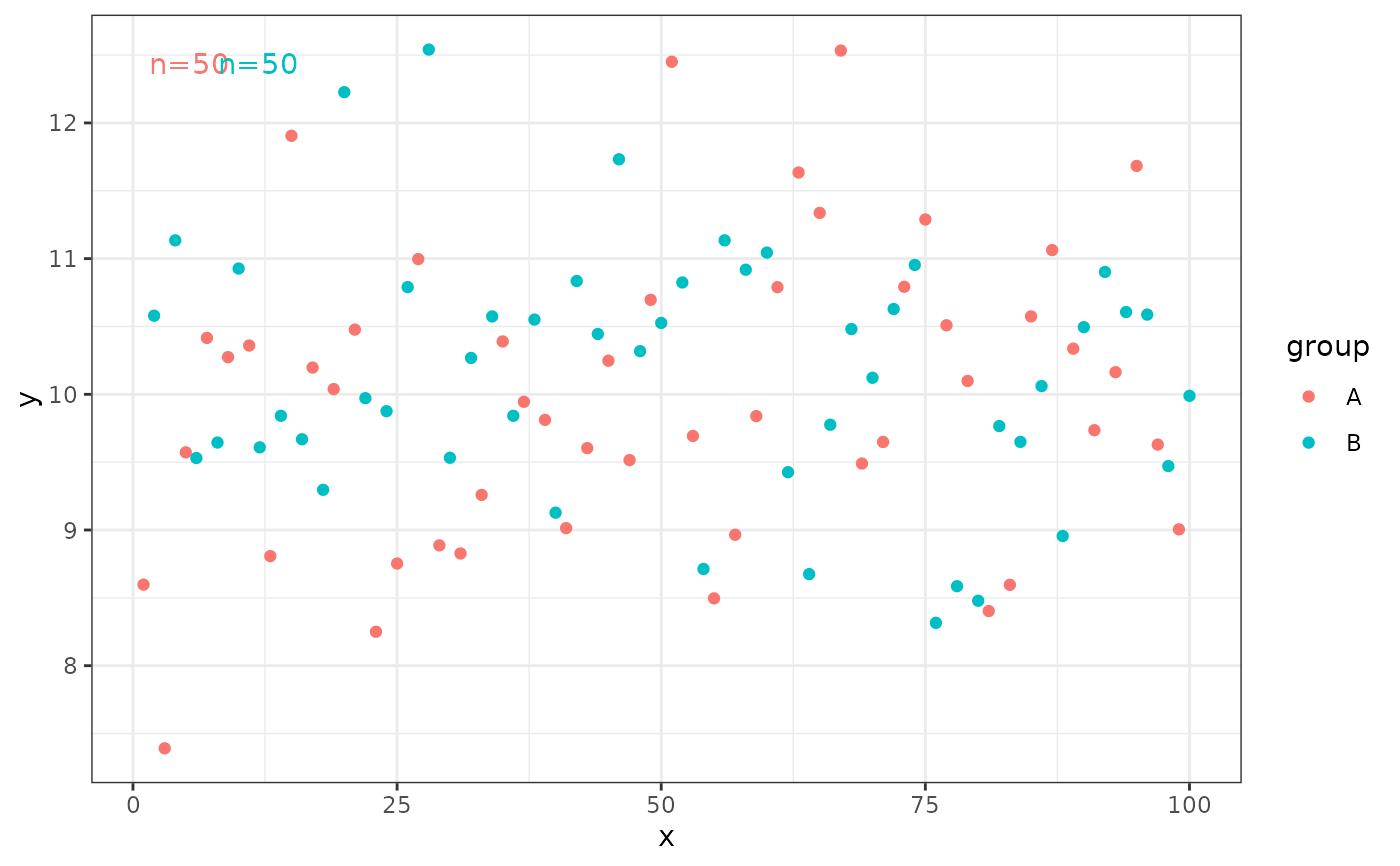
 ggplot(my.data, aes(x, y, colour = group)) +
geom_point() +
stat_group_counts(label.x = "left", hstep = 0.06, vstep = 0)
ggplot(my.data, aes(x, y, colour = group)) +
geom_point() +
stat_group_counts(label.x = "left", hstep = 0.06, vstep = 0)
 ggplot(my.data, aes(x, y, colour = group)) +
geom_point() +
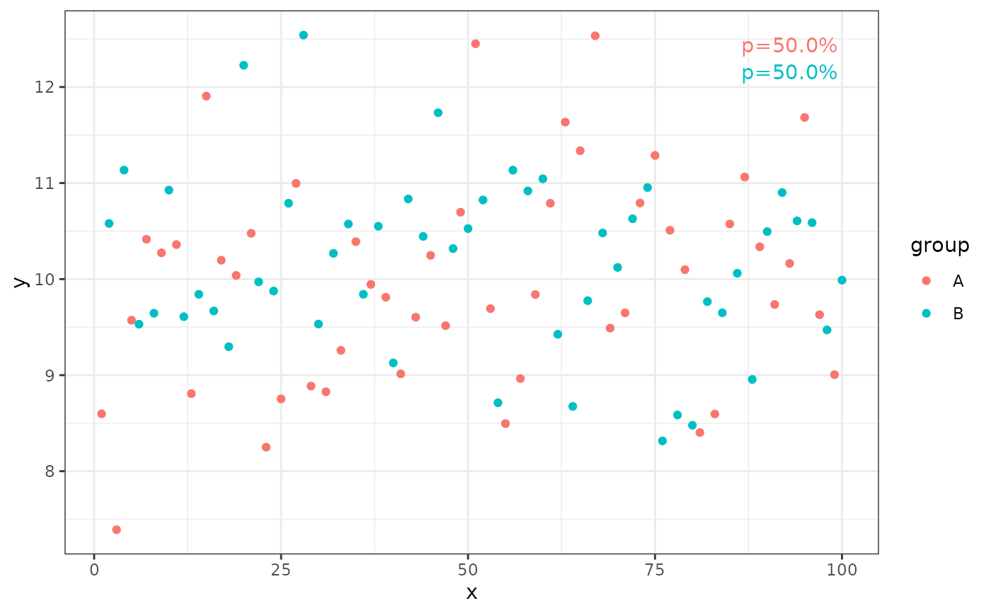
stat_group_counts(aes(label = after_stat(pc.label)))
ggplot(my.data, aes(x, y, colour = group)) +
geom_point() +
stat_group_counts(aes(label = after_stat(pc.label)))
 ggplot(my.data, aes(x, y, colour = group)) +
geom_point() +
stat_group_counts(aes(label = after_stat(pc.label)), digits = 3)
ggplot(my.data, aes(x, y, colour = group)) +
geom_point() +
stat_group_counts(aes(label = after_stat(pc.label)), digits = 3)
 ggplot(my.data, aes(x, y, colour = group)) +
geom_point() +
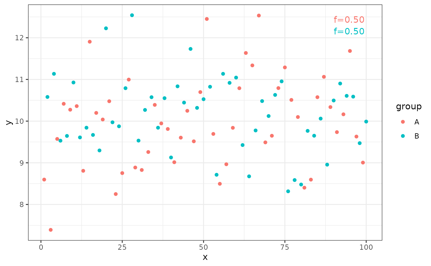
stat_group_counts(aes(label = after_stat(fr.label)))
ggplot(my.data, aes(x, y, colour = group)) +
geom_point() +
stat_group_counts(aes(label = after_stat(fr.label)))
 ggplot(my.data, aes(x, y, colour = group)) +
geom_point() +
stat_group_counts(aes(label = after_stat(dec.label)))
ggplot(my.data, aes(x, y, colour = group)) +
geom_point() +
stat_group_counts(aes(label = after_stat(dec.label)))
 # one of x or y can be a factor
# label.x or label.y along the factor can be set to "factor" together
# with the use of geom_text()
ggplot(mpg,
aes(factor(cyl), hwy)) +
stat_boxplot() +
stat_group_counts(geom = "text",
label.y = 10,
label.x = "factor") +
stat_panel_counts()
# one of x or y can be a factor
# label.x or label.y along the factor can be set to "factor" together
# with the use of geom_text()
ggplot(mpg,
aes(factor(cyl), hwy)) +
stat_boxplot() +
stat_group_counts(geom = "text",
label.y = 10,
label.x = "factor") +
stat_panel_counts()
 # Numeric values can be used to build labels with alternative formats
# Here with sprintf(), but paste() and format() also work.
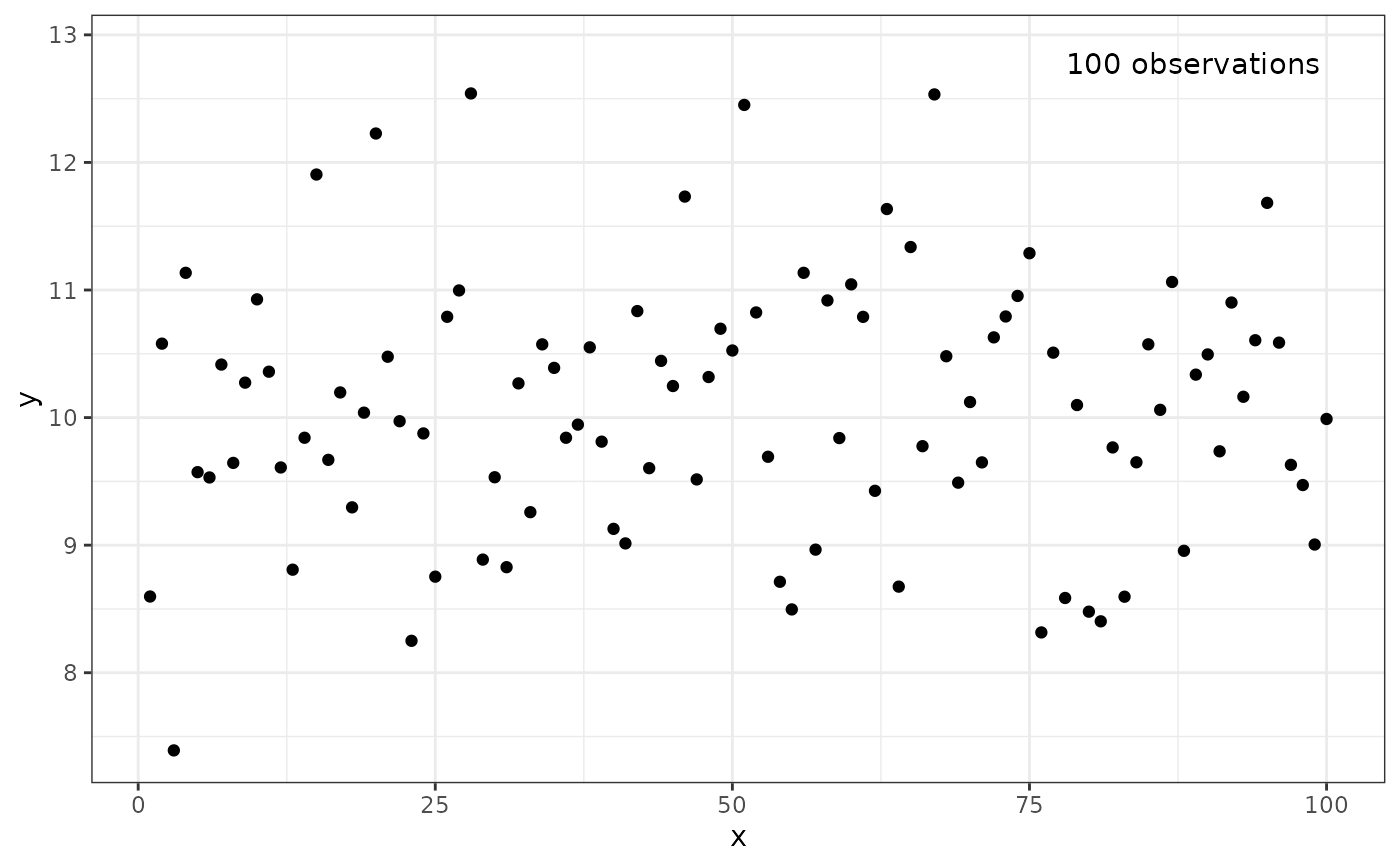
ggplot(my.data, aes(x, y)) +
geom_point() +
stat_panel_counts(aes(label = sprintf("%i observations",
after_stat(count)))) +
scale_y_continuous(expand = expansion(mult = c(0.05, 0.12)))
# Numeric values can be used to build labels with alternative formats
# Here with sprintf(), but paste() and format() also work.
ggplot(my.data, aes(x, y)) +
geom_point() +
stat_panel_counts(aes(label = sprintf("%i observations",
after_stat(count)))) +
scale_y_continuous(expand = expansion(mult = c(0.05, 0.12)))
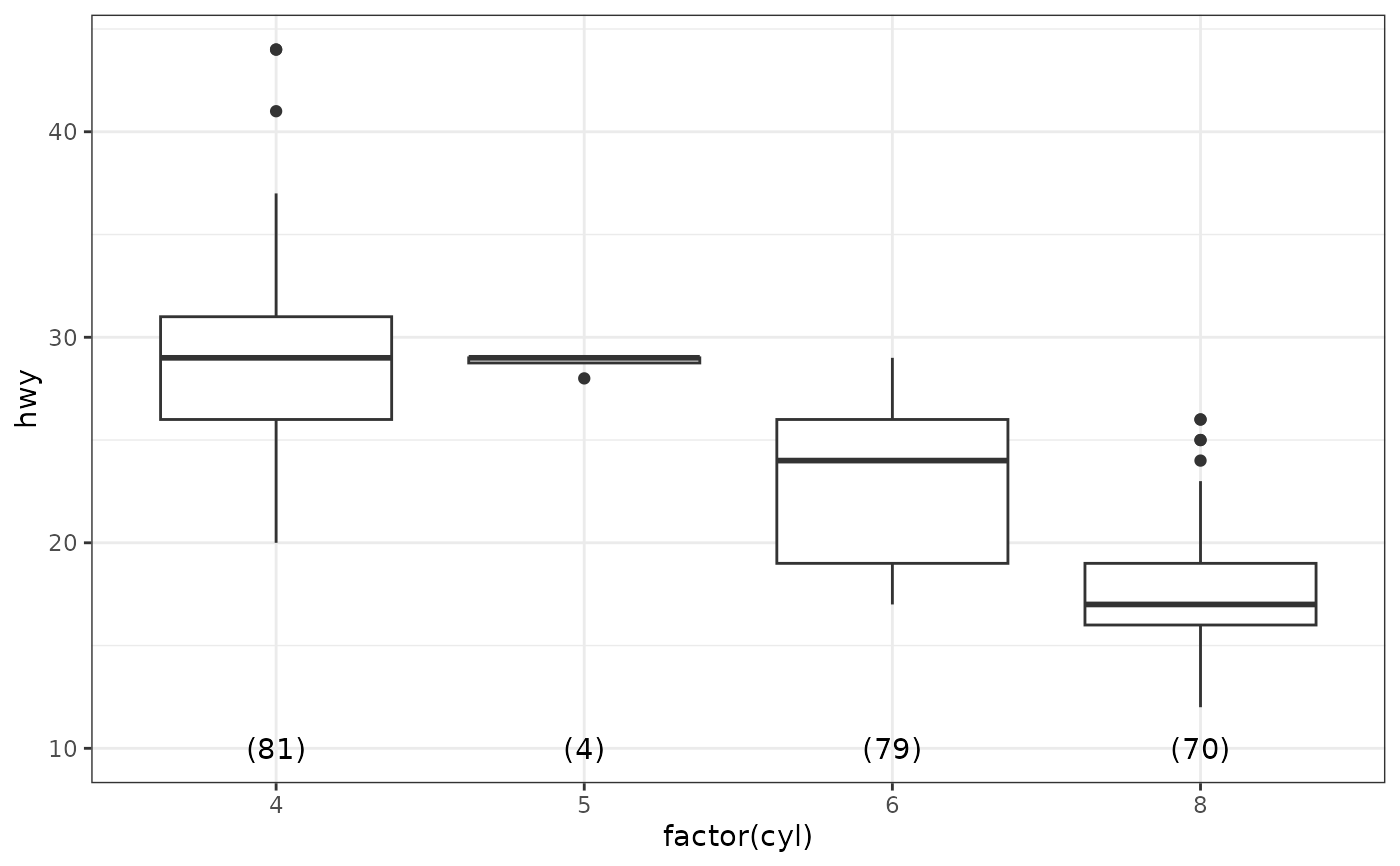
 ggplot(mpg,
aes(factor(cyl), hwy)) +
stat_boxplot() +
stat_group_counts(geom = "text",
aes(label = sprintf("(%i)", after_stat(count))),
label.y = 10,
label.x = "factor")
ggplot(mpg,
aes(factor(cyl), hwy)) +
stat_boxplot() +
stat_group_counts(geom = "text",
aes(label = sprintf("(%i)", after_stat(count))),
label.y = 10,
label.x = "factor")
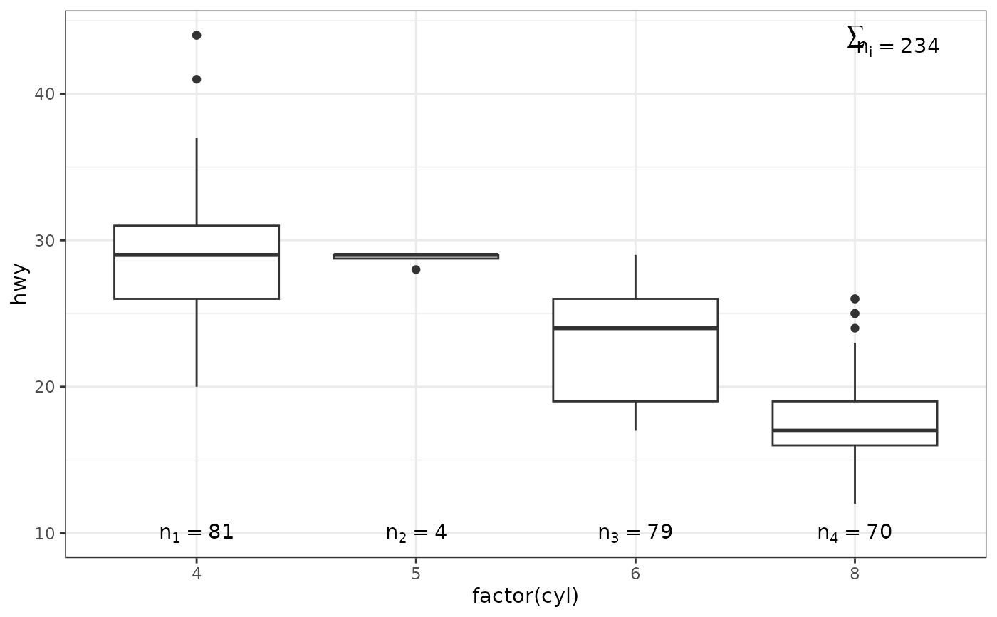
 ggplot(mpg,
aes(factor(cyl), hwy)) +
stat_boxplot() +
stat_group_counts(aes(label = sprintf("n[%i]~`=`~%i",
after_stat(x), after_stat(count))),
parse = TRUE,
geom = "text",
label.y = 10,
label.x = "factor") +
stat_panel_counts(aes(label = sprintf("sum(n[i])~`=`~%i",
after_stat(count))),
parse = TRUE)
ggplot(mpg,
aes(factor(cyl), hwy)) +
stat_boxplot() +
stat_group_counts(aes(label = sprintf("n[%i]~`=`~%i",
after_stat(x), after_stat(count))),
parse = TRUE,
geom = "text",
label.y = 10,
label.x = "factor") +
stat_panel_counts(aes(label = sprintf("sum(n[i])~`=`~%i",
after_stat(count))),
parse = TRUE)
 # label position
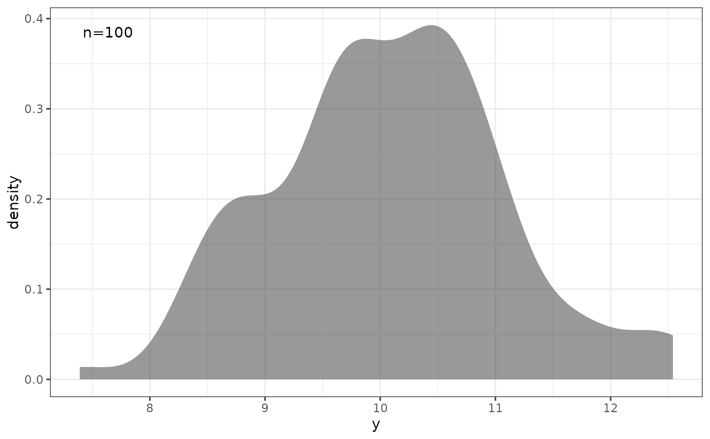
ggplot(my.data, aes(y)) +
stat_panel_counts(label.x = "left") +
stat_density(alpha = 0.5)
# label position
ggplot(my.data, aes(y)) +
stat_panel_counts(label.x = "left") +
stat_density(alpha = 0.5)
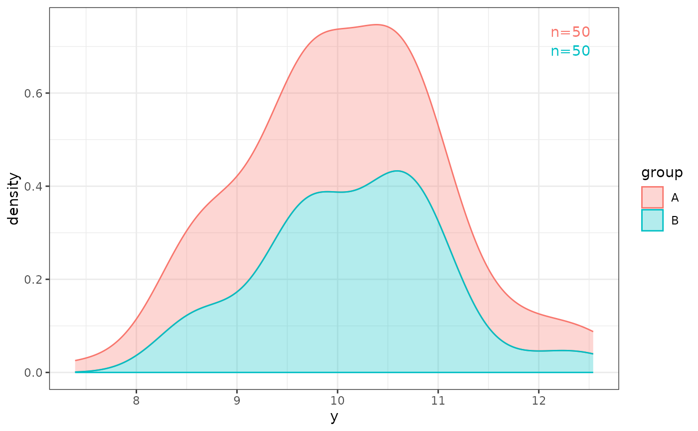
 ggplot(my.data, aes(y, colour = group)) +
stat_group_counts(label.y = "top") +
stat_density(aes(fill = group), alpha = 0.3)
ggplot(my.data, aes(y, colour = group)) +
stat_group_counts(label.y = "top") +
stat_density(aes(fill = group), alpha = 0.3)
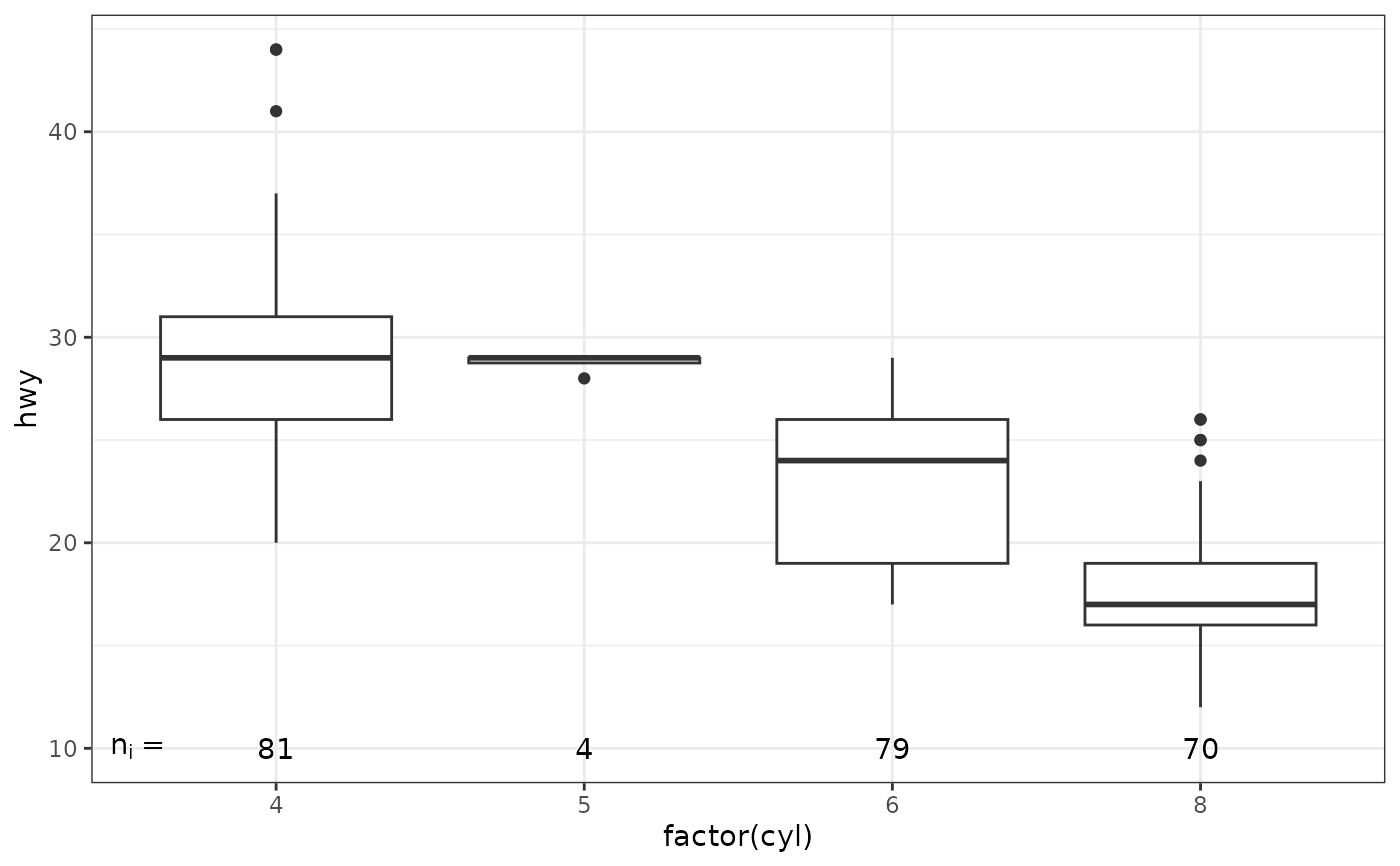
 # The numeric value can be used as a label as is
ggplot(mpg,
aes(factor(cyl), hwy)) +
stat_boxplot() +
stat_group_counts(geom = "text",
aes(label = after_stat(count)),
label.x = "factor",
label.y = 10) +
annotate(geom = "text", x = 0.55, y = 10, label = "n[i]~`=`", parse = TRUE)
# The numeric value can be used as a label as is
ggplot(mpg,
aes(factor(cyl), hwy)) +
stat_boxplot() +
stat_group_counts(geom = "text",
aes(label = after_stat(count)),
label.x = "factor",
label.y = 10) +
annotate(geom = "text", x = 0.55, y = 10, label = "n[i]~`=`", parse = TRUE)
 # We use geom_debug() to see the computed values
gginnards.installed <- requireNamespace("gginnards", quietly = TRUE)
if (gginnards.installed) {
library(gginnards)
ggplot(my.data, aes(x, y)) +
geom_point() +
stat_panel_counts(geom = "debug")
}
# We use geom_debug() to see the computed values
gginnards.installed <- requireNamespace("gginnards", quietly = TRUE)
if (gginnards.installed) {
library(gginnards)
ggplot(my.data, aes(x, y)) +
geom_point() +
stat_panel_counts(geom = "debug")
}
 #> [1] "PANEL 1; group(s) NULL; 'draw_function()' input 'data' (head):"
#> npcx npcy label PANEL x y count count.label
#> 1 NA NA n=100 1 95.05 12.28333 100 n=100
if (gginnards.installed) {
ggplot(my.data, aes(x, y, colour = group)) +
geom_point() +
stat_group_counts(geom = "debug")
}
#> [1] "PANEL 1; group(s) NULL; 'draw_function()' input 'data' (head):"
#> npcx npcy label PANEL x y count count.label
#> 1 NA NA n=100 1 95.05 12.28333 100 n=100
if (gginnards.installed) {
ggplot(my.data, aes(x, y, colour = group)) +
geom_point() +
stat_group_counts(geom = "debug")
}
 #> [1] "PANEL 1; group(s) 1, 2; 'draw_function()' input 'data' (head):"
#> colour npcx npcy label x y PANEL group count total count.label
#> 1 #F8766D NA NA n=50 100 12.54082 1 1 50 100 n=50
#> 2 #00BFC4 NA NA n=50 100 12.28333 1 2 50 100 n=50
#> pc.label dec.label fr.label
#> 1 p=50% f=0.50 50 / 100
#> 2 p=50% f=0.50 50 / 100
#> [1] "PANEL 1; group(s) 1, 2; 'draw_function()' input 'data' (head):"
#> colour npcx npcy label x y PANEL group count total count.label
#> 1 #F8766D NA NA n=50 100 12.54082 1 1 50 100 n=50
#> 2 #00BFC4 NA NA n=50 100 12.28333 1 2 50 100 n=50
#> pc.label dec.label fr.label
#> 1 p=50% f=0.50 50 / 100
#> 2 p=50% f=0.50 50 / 100