stat_dens2d_filter Filters-out/filters-in observations in
regions of a plot panel with high density of observations, based on the
values mapped to both x and y aesthetics.
stat_dens2d_filter_g does the filtering by group instead of by
panel. This second stat is useful for highlighting observations, while the
first one tends to be most useful when the aim is to prevent clashes among
text labels. If there is no mapping to label in data, the
mapping is silently set to rownames(data).
stat_dens2d_filter(
  mapping = NULL,
  data = NULL,
  geom = "point",
  position = "identity",
  ...,
  keep.fraction = 0.1,
  keep.number = Inf,
  keep.sparse = TRUE,
  keep.these = FALSE,
  exclude.these = FALSE,
  these.target = "label",
  pool.along = c("xy", "x", "y", "none"),
  xintercept = 0,
  yintercept = 0,
  invert.selection = FALSE,
  na.rm = TRUE,
  show.legend = FALSE,
  inherit.aes = TRUE,
  h = NULL,
  n = NULL,
  return.density = FALSE
)

stat_dens2d_filter_g(
  mapping = NULL,
  data = NULL,
  geom = "point",
  position = "identity",
  ...,
  keep.fraction = 0.1,
  keep.number = Inf,
  keep.sparse = TRUE,
  keep.these = FALSE,
  exclude.these = FALSE,
  these.target = "label",
  pool.along = c("xy", "x", "y", "none"),
  xintercept = 0,
  yintercept = 0,
  invert.selection = FALSE,
  na.rm = TRUE,
  show.legend = FALSE,
  inherit.aes = TRUE,
  h = NULL,
  n = NULL,
  return.density = FALSE
)
Arguments
- mapping
The aesthetic mapping, usually constructed with
aesoraes_. Only needs to be set at the layer level if you are overriding the plot defaults.- data
A layer specific dataset - only needed if you want to override the plot defaults.
- geom
The geometric object to use display the data.
- position
The position adjustment to use for overlapping points on this layer
- ...
other arguments passed on to
layer. This can include aesthetics whose values you want to set, not map. Seelayerfor more details.- keep.fraction
numeric [0..1]. The fraction of the observations (or rows) in
datato be retained.- keep.number
integer Set the maximum number of observations to retain, effective only if obeying
keep.fractionwould result in a larger number.- keep.sparse
logical If
TRUE, the default, observations from the more sparse regions are retained, ifFALSEthose from the densest regions.- keep.these, exclude.these
character vector, integer vector, logical vector or function that takes one or more variables in data selected by
these.target. Negative integers behave as in R's extraction methods. The rows fromdataindicated bykeep.theseandexclude.theseare kept or excluded irrespective of the local density.- these.target
character, numeric or logical selecting one or more column(s) of
data. IfTRUEthe wholedataobject is passed.- pool.along
character, one of
"none","x","y", or"xy"indicating if selection should be done pooling the observations along the x,y, both axes or none based on quadrants given byxinterceptandyintercept.- xintercept, yintercept
numeric The center point of the quadrants.
- invert.selection
logical If
TRUE, the complement of the selected rows are returned.- na.rm
a logical value indicating whether NA values should be stripped before the computation proceeds.
- show.legend
logical. Should this layer be included in the legends?
NA, the default, includes if any aesthetics are mapped.FALSEnever includes, andTRUEalways includes.- inherit.aes
If
FALSE, overrides the default aesthetics, rather than combining with them. This is most useful for helper functions that define both data and aesthetics and shouldn't inherit behaviour from the default plot specification, e.g.borders.- h
vector of bandwidths for x and y directions. Defaults to normal reference bandwidth (see bandwidth.nrd). A scalar value will be taken to apply to both directions.
- n
Number of grid points in each direction. Can be scalar or a length-2 integer vector
- return.density
logical vector of lenght 1. If
TRUEadd columns"density"and"keep.obs"to the returned data frame.
Value
A plot layer instance. Using as output data a subset of the
rows in input data retained based on a 2D-density-based filtering
criterion.
Details
The local density of observations in 2D (x and y) is
computed with function kde2d and used to select
observations, passing to the geom a subset of the rows in its data
input. The default is to select observations in sparse regions of the plot,
but the selection can be inverted so that only observations in the densest
regions are returned. Specific observations can be protected from being
deselected and "kept" by passing a suitable argument to keep.these.
Logical and integer vectors work as indexes to rows in data, while a
character vector values are compared to the character values mapped to the
label aesthetic. A function passed as argument to keep.these will
receive as argument the values in the variable mapped to label and
should return a character, logical or numeric vector as described above. If
no variable has been mapped to label, row names are used in its
place.
How many rows are retained in addition to those in keep.these is
controlled with arguments passed to keep.number and
keep.fraction. keep.number sets the maximum number of
observations selected, whenever keep.fraction results in fewer
observations selected, it is obeyed.
Computation of density and of the default bandwidth require at least
two observations with different values. If data do not fulfill this
condition, they are kept only if keep.fraction = 1. This is correct
behavior for a single observation, but can be surprising in the case of
multiple observations.
Parameters keep.these and exclude.these make it possible to
force inclusion or exclusion of observations after the density is computed.
In case of conflict, exclude.these overrides keep.these.
Note
Which points are kept and which not depends on how dense a grid is used
and how flexible the density surface estimate is. This depends on the
values passed as arguments to parameters n, bw and
kernel. It is also important to be aware that both
geom_text() and geom_text_repel() can avoid overplotting by
discarding labels at the plot rendering stage, i.e., what is plotted may
differ from what is returned by this statistic.
See also
stat_dens2d_labels and kde2d used
internally. Parameters n, h in these statistics correspond to
the parameters with the same name in this imported function. Limits are set
to the limits of the plot scales.
Other statistics returning a subset of data:
stat_dens1d_filter(),
stat_dens1d_labels(),
stat_dens2d_labels()
Examples
random_string <-
function(len = 6) {
paste(sample(letters, len, replace = TRUE), collapse = "")
}
# Make random data.
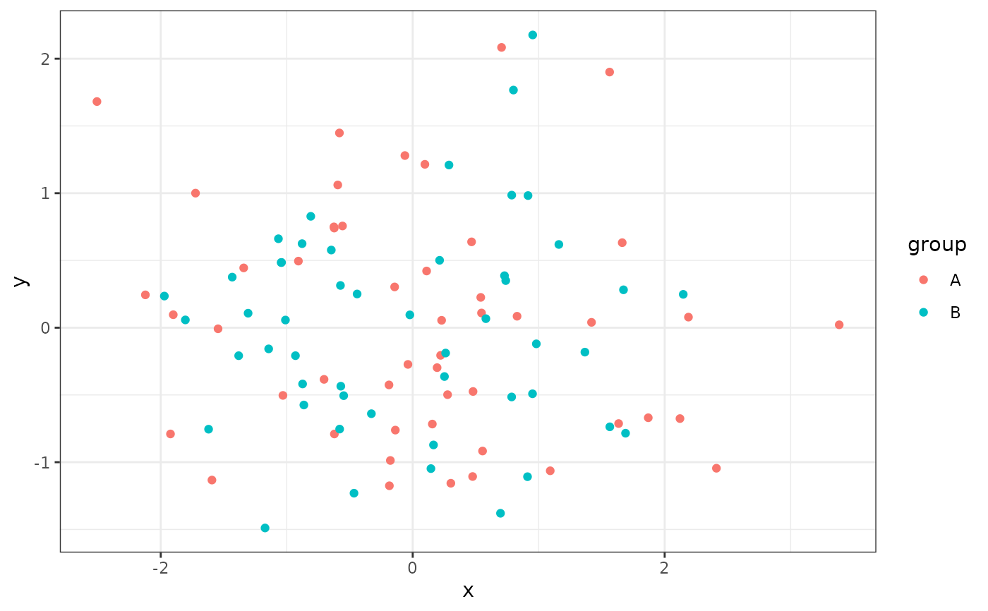
set.seed(1001)
d <- tibble::tibble(
x = rnorm(100),
y = rnorm(100),
group = rep(c("A", "B"), c(50, 50)),
lab = replicate(100, { random_string() })
)
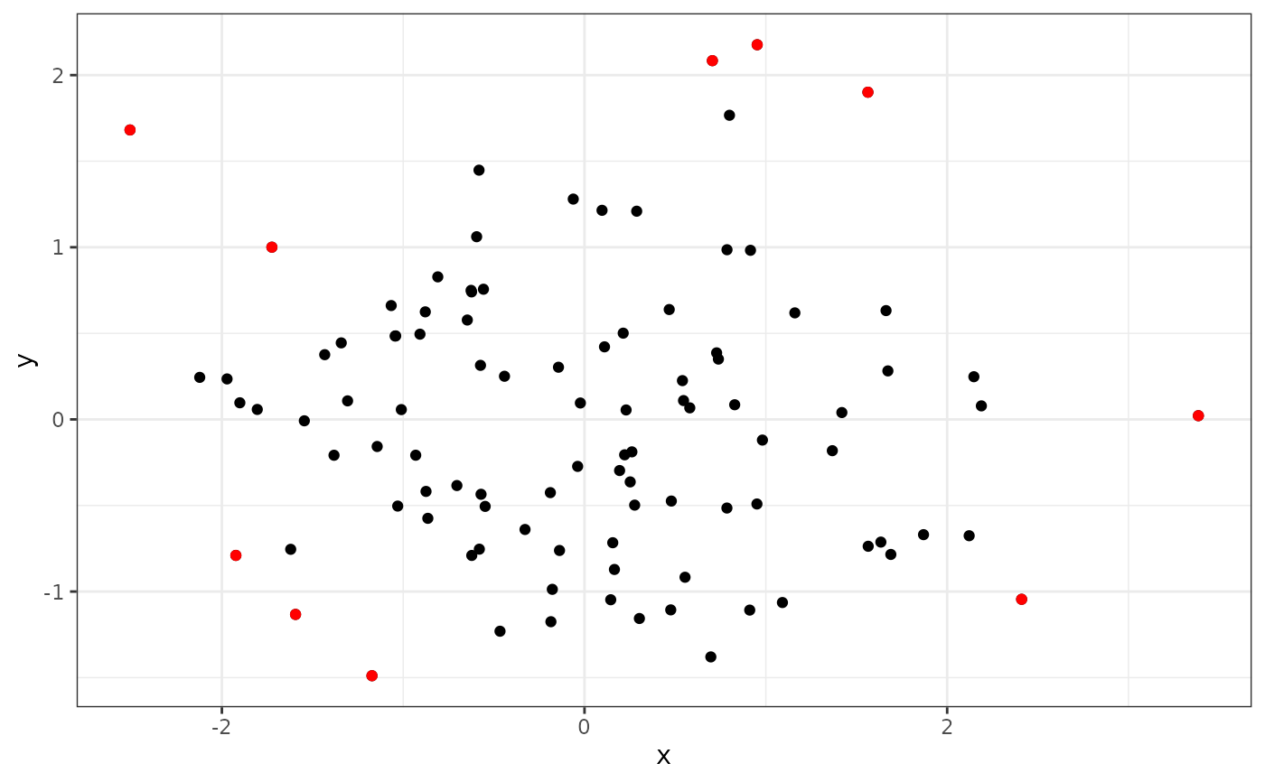
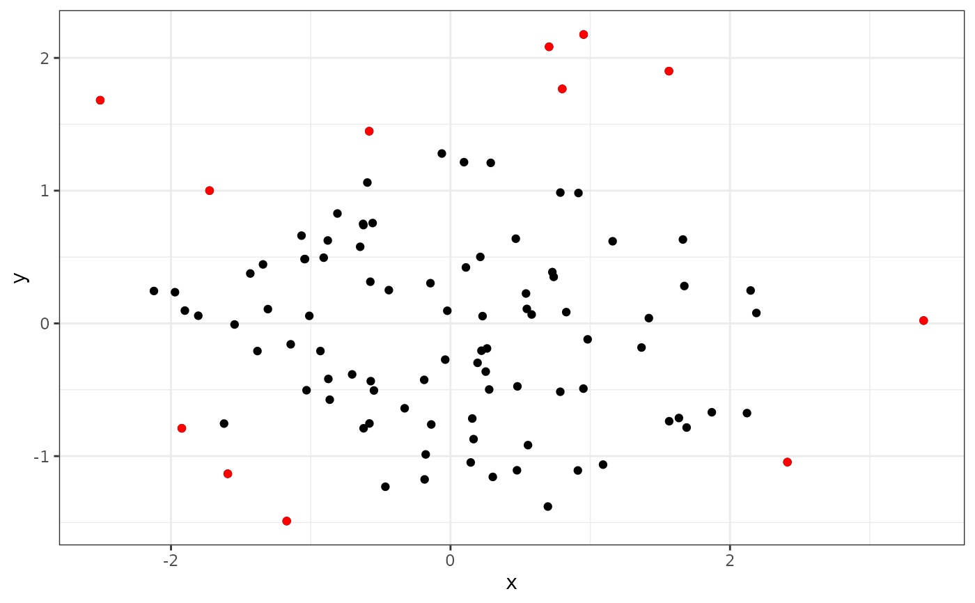
# filter (and here highlight) 1/10 observations in sparsest regions
ggplot(data = d, aes(x, y)) +
geom_point() +
stat_dens2d_filter(colour = "red")
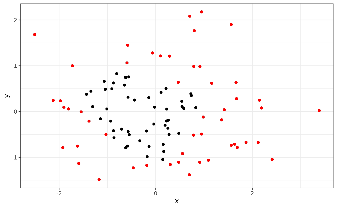
 # filter observations not in the sparsest regions
ggplot(data = d, aes(x, y)) +
geom_point() +
stat_dens2d_filter(colour = "blue", invert.selection = TRUE)
# filter observations not in the sparsest regions
ggplot(data = d, aes(x, y)) +
geom_point() +
stat_dens2d_filter(colour = "blue", invert.selection = TRUE)
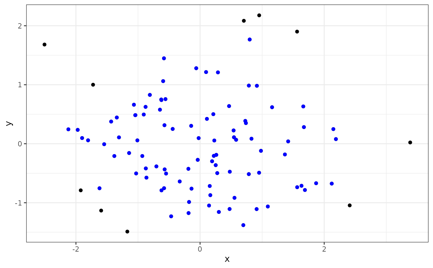 # filter observations in dense regions of the plot
ggplot(data = d, aes(x, y)) +
geom_point() +
stat_dens2d_filter(colour = "blue", keep.sparse = FALSE)
# filter observations in dense regions of the plot
ggplot(data = d, aes(x, y)) +
geom_point() +
stat_dens2d_filter(colour = "blue", keep.sparse = FALSE)
 # filter 1/2 the observations
ggplot(data = d, aes(x, y)) +
geom_point() +
stat_dens2d_filter(colour = "red", keep.fraction = 0.5)
# filter 1/2 the observations
ggplot(data = d, aes(x, y)) +
geom_point() +
stat_dens2d_filter(colour = "red", keep.fraction = 0.5)
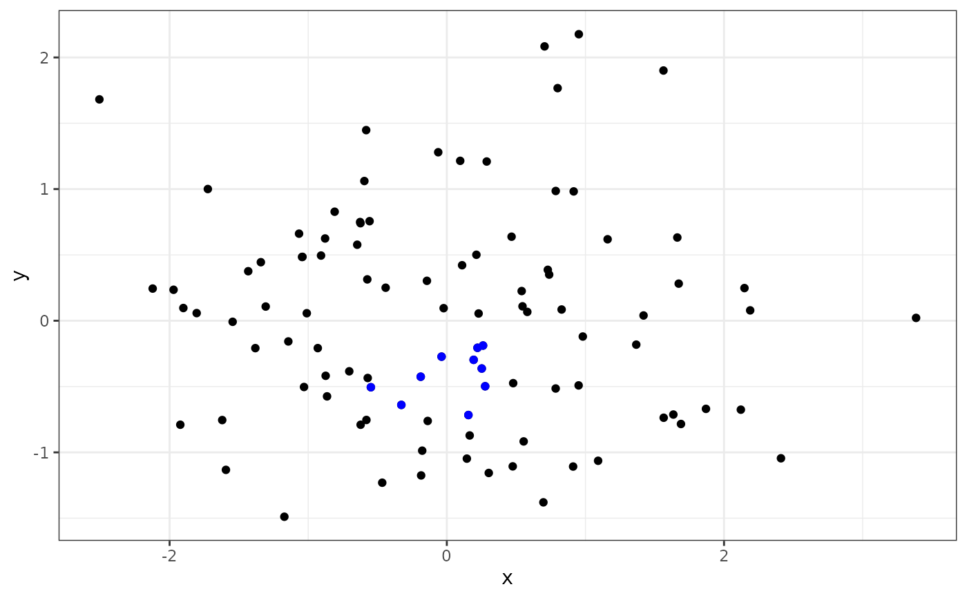
 # filter 1/2 the observations but cap their number to maximum 12 observations
ggplot(data = d, aes(x, y)) +
geom_point() +
stat_dens2d_filter(colour = "red",
keep.fraction = 0.5,
keep.number = 12)
# filter 1/2 the observations but cap their number to maximum 12 observations
ggplot(data = d, aes(x, y)) +
geom_point() +
stat_dens2d_filter(colour = "red",
keep.fraction = 0.5,
keep.number = 12)
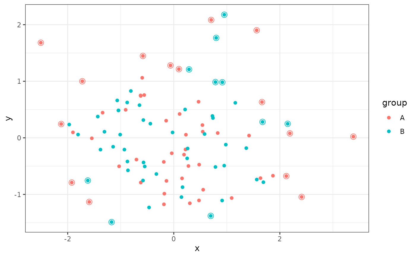
 # density filtering done jointly across groups
ggplot(data = d, aes(x, y, colour = group)) +
geom_point() +
stat_dens2d_filter(shape = 1, size = 3, keep.fraction = 1/4)
# density filtering done jointly across groups
ggplot(data = d, aes(x, y, colour = group)) +
geom_point() +
stat_dens2d_filter(shape = 1, size = 3, keep.fraction = 1/4)
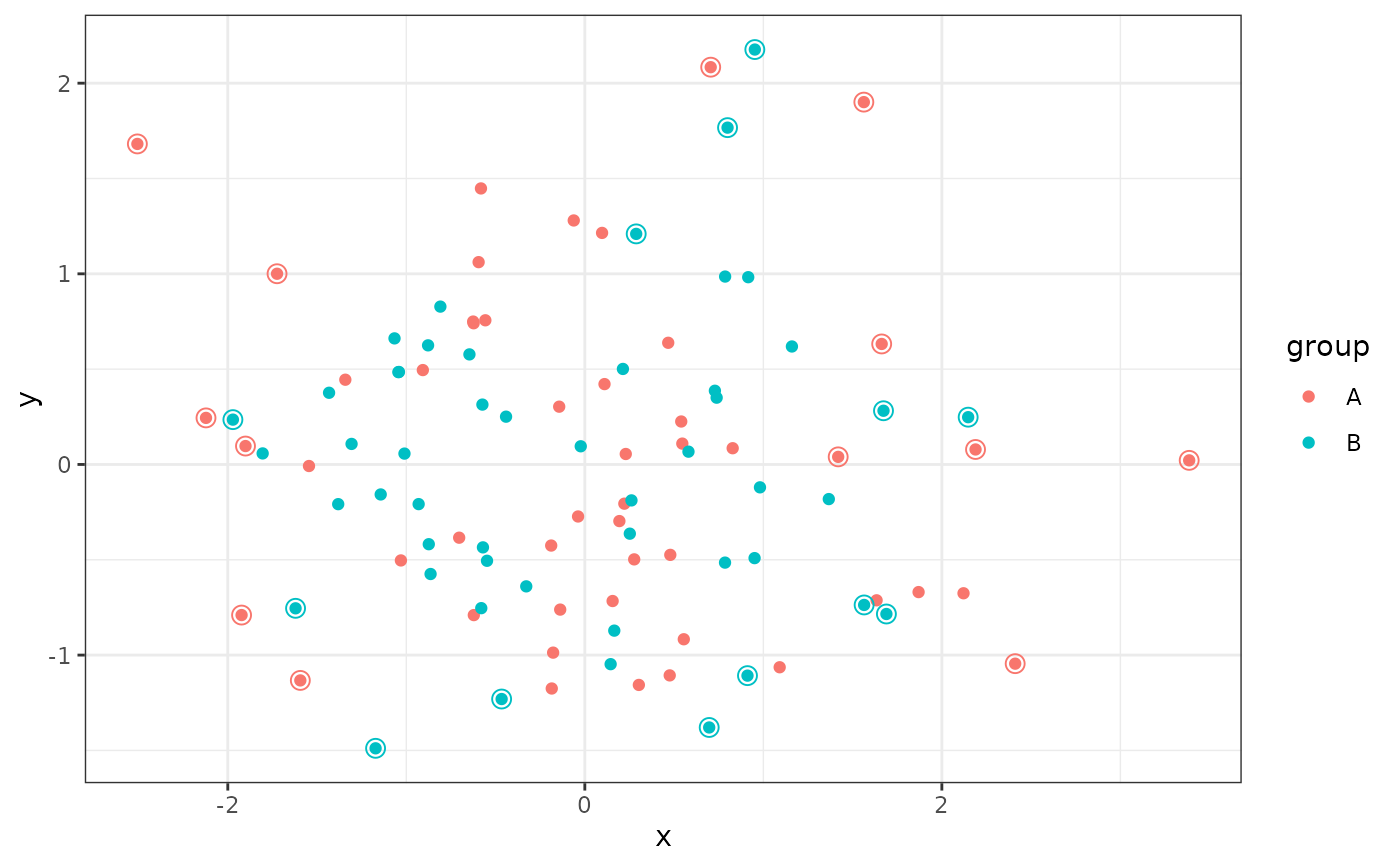
 # density filtering done independently for each group
ggplot(data = d, aes(x, y, colour = group)) +
geom_point() +
stat_dens2d_filter_g(shape = 1, size = 3, keep.fraction = 1/4)
# density filtering done independently for each group
ggplot(data = d, aes(x, y, colour = group)) +
geom_point() +
stat_dens2d_filter_g(shape = 1, size = 3, keep.fraction = 1/4)
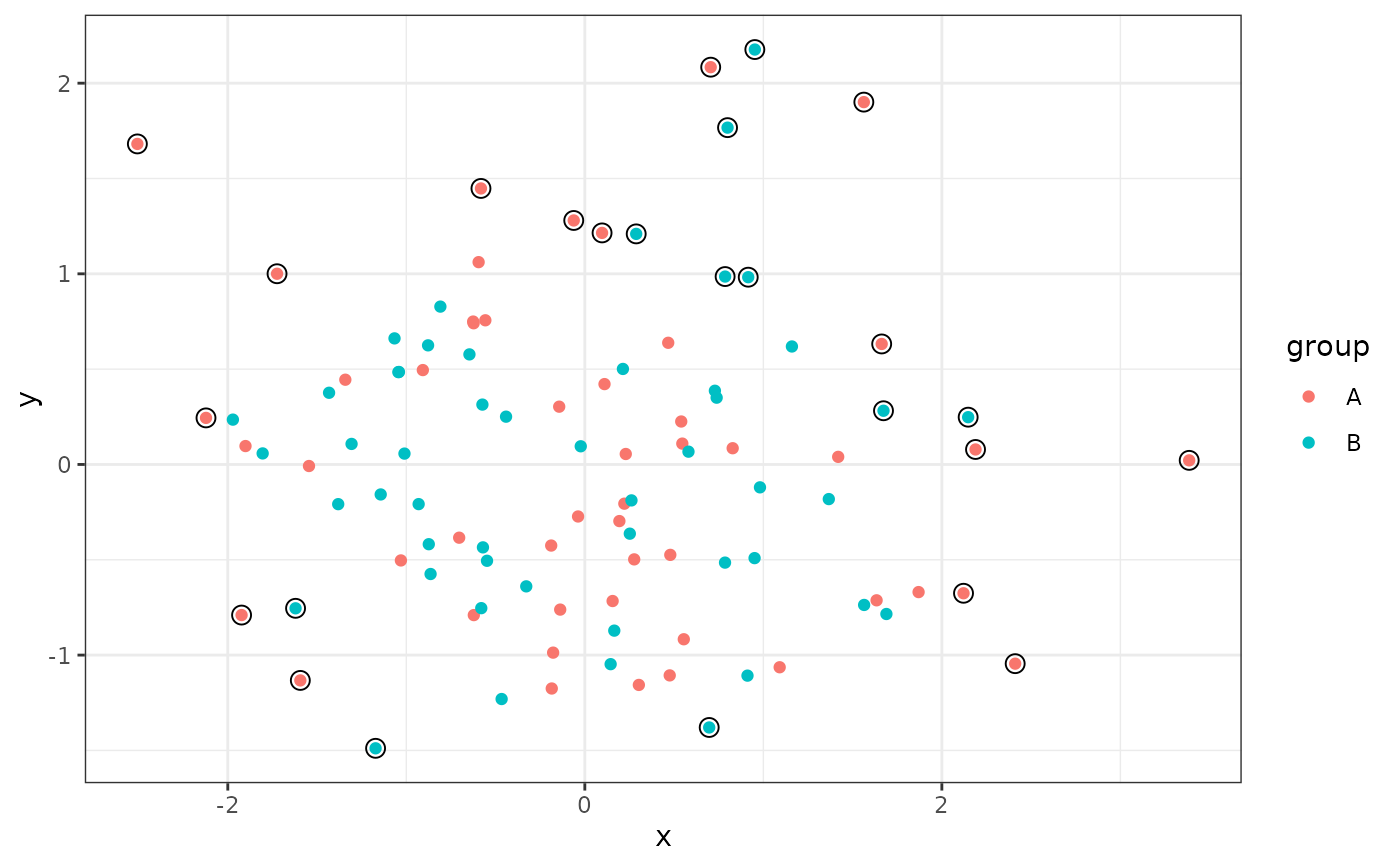
 # density filtering done jointly across groups by overriding grouping
ggplot(data = d, aes(x, y, colour = group)) +
geom_point() +
stat_dens2d_filter_g(colour = "black",
shape = 1, size = 3, keep.fraction = 1/4)
# density filtering done jointly across groups by overriding grouping
ggplot(data = d, aes(x, y, colour = group)) +
geom_point() +
stat_dens2d_filter_g(colour = "black",
shape = 1, size = 3, keep.fraction = 1/4)
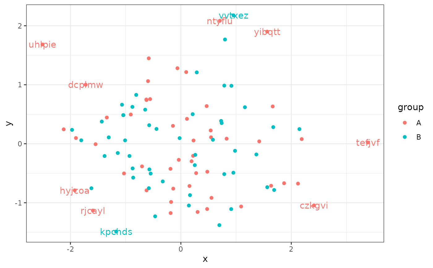
 # label observations
ggplot(data = d, aes(x, y, label = lab, colour = group)) +
geom_point() +
stat_dens2d_filter(geom = "text")
# label observations
ggplot(data = d, aes(x, y, label = lab, colour = group)) +
geom_point() +
stat_dens2d_filter(geom = "text")
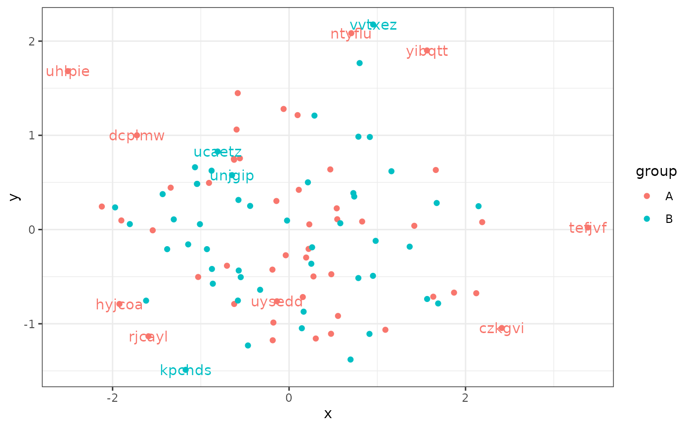
 ggplot(data = d, aes(x, y, label = lab, colour = group)) +
geom_point() +
stat_dens2d_filter(geom = "text",
keep.these = function(x) {grepl("^u", x)})
ggplot(data = d, aes(x, y, label = lab, colour = group)) +
geom_point() +
stat_dens2d_filter(geom = "text",
keep.these = function(x) {grepl("^u", x)})
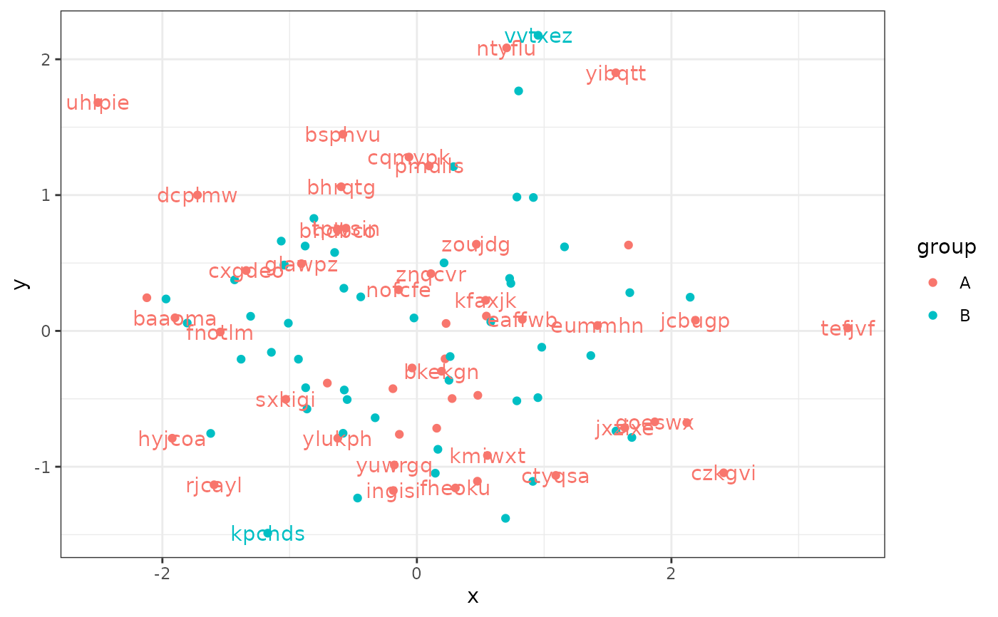
 ggplot(data = d, aes(x, y, label = lab, colour = group)) +
geom_point() +
stat_dens2d_filter(geom = "text",
keep.these = 1:30)
ggplot(data = d, aes(x, y, label = lab, colour = group)) +
geom_point() +
stat_dens2d_filter(geom = "text",
keep.these = 1:30)
 # looking under the hood with gginnards::geom_debug()
gginnards.installed <- requireNamespace("gginnards", quietly = TRUE)
if (gginnards.installed) {
library(gginnards)
ggplot(data = d, aes(x, y, label = lab, colour = group)) +
stat_dens2d_filter(geom = "debug")
ggplot(data = d, aes(x, y, label = lab, colour = group)) +
geom_point() +
stat_dens2d_filter(geom = "debug", return.density = TRUE)
}
# looking under the hood with gginnards::geom_debug()
gginnards.installed <- requireNamespace("gginnards", quietly = TRUE)
if (gginnards.installed) {
library(gginnards)
ggplot(data = d, aes(x, y, label = lab, colour = group)) +
stat_dens2d_filter(geom = "debug")
ggplot(data = d, aes(x, y, label = lab, colour = group)) +
geom_point() +
stat_dens2d_filter(geom = "debug", return.density = TRUE)
}
 #> [1] "PANEL 1; group(s) 1, 2; 'draw_function()' input 'data' (head):"
#> colour x y label PANEL group keep.obs density
#> 1 #F8766D -2.5065362 1.6814089 uhlpie 1 1 TRUE 0.01009701
#> 2 #F8766D -1.5937133 -1.1328282 rjcayl 1 1 TRUE 0.02714959
#> 3 #F8766D 1.5629506 1.9006755 yibqtt 1 1 TRUE 0.01839611
#> 4 #F8766D 2.4107390 -1.0449415 czkgvi 1 1 TRUE 0.02392334
#> 5 #F8766D -1.9227946 -0.7900107 hyjcoa 1 1 TRUE 0.02708956
#> 6 #F8766D 0.7051636 2.0839521 ntyflu 1 1 TRUE 0.02646842
#> xintercept yintercept
#> 1 0 0
#> 2 0 0
#> 3 0 0
#> 4 0 0
#> 5 0 0
#> 6 0 0
#> [1] "PANEL 1; group(s) 1, 2; 'draw_function()' input 'data' (head):"
#> colour x y label PANEL group keep.obs density
#> 1 #F8766D -2.5065362 1.6814089 uhlpie 1 1 TRUE 0.01009701
#> 2 #F8766D -1.5937133 -1.1328282 rjcayl 1 1 TRUE 0.02714959
#> 3 #F8766D 1.5629506 1.9006755 yibqtt 1 1 TRUE 0.01839611
#> 4 #F8766D 2.4107390 -1.0449415 czkgvi 1 1 TRUE 0.02392334
#> 5 #F8766D -1.9227946 -0.7900107 hyjcoa 1 1 TRUE 0.02708956
#> 6 #F8766D 0.7051636 2.0839521 ntyflu 1 1 TRUE 0.02646842
#> xintercept yintercept
#> 1 0 0
#> 2 0 0
#> 3 0 0
#> 4 0 0
#> 5 0 0
#> 6 0 0