stat_dens1d_labels() Sets values mapped to the
label aesthetic to "" or a user provided character string
based on the local density in regions of a plot panel. Its main use is
together with repulsive geoms from package ggrepel
to restrict labeling to the low density tails of a distribution. By default
the data are handled all together, but it is also possible to control
labeling separately in each tail.
If there is no mapping to label in data, the mapping is set
to rownames(data), with a message.
stat_dens1d_labels(
  mapping = NULL,
  data = NULL,
  geom = "text",
  position = "identity",
  ...,
  keep.fraction = 0.1,
  keep.number = Inf,
  keep.sparse = TRUE,
  keep.these = FALSE,
  exclude.these = FALSE,
  these.target = "label",
  pool.along = c("x", "none"),
  xintercept = 0,
  invert.selection = FALSE,
  bw = "SJ",
  kernel = "gaussian",
  adjust = 1,
  n = 512,
  orientation = c("x", "y"),
  label.fill = "",
  return.density = FALSE,
  na.rm = TRUE,
  show.legend = FALSE,
  inherit.aes = TRUE
)
Arguments
- mapping
The aesthetic mapping, usually constructed with
aesoraes_. Only needs to be set at the layer level if you are overriding the plot defaults.- data
A layer specific dataset - only needed if you want to override the plot defaults.
- geom
The geometric object to use display the data.
- position
The position adjustment to use for overlapping points on this layer
- ...
other arguments passed on to
layer. This can include aesthetics whose values you want to set, not map. Seelayerfor more details.- keep.fraction
numeric vector of length 1 or 2 [0..1]. The fraction of the observations (or rows) in
datato be retained.- keep.number
integer vector of length 1 or 2. Set the maximum number of observations to retain, effective only if obeying
keep.fractionwould result in a larger number.- keep.sparse
logical If
TRUE, the default, observations from the more sparse regions are retained, ifFALSEthose from the densest regions.- keep.these, exclude.these
character vector, integer vector, logical vector or function that takes one or more variables in data selected by
these.target. Negative integers behave as in R's extraction methods. The rows fromdataindicated bykeep.theseandexclude.theseare kept or excluded irrespective of the local density.- these.target
character, numeric or logical selecting one or more column(s) of
data. IfTRUEthe wholedataobject is passed.- pool.along
character, one of
"none"or"x", indicating if selection should be done pooling the observations along the x aesthetic, or separately on either side ofxintercept.- xintercept
numeric The split point for the data filtering.
- invert.selection
logical If
TRUE, the complement of the selected rows are returned.- bw
numeric or character The smoothing bandwidth to be used. If numeric, the standard deviation of the smoothing kernel. If character, a rule to choose the bandwidth, as listed in
bw.nrd.- kernel
character See
densityfor details.- adjust
numeric A multiplicative bandwidth adjustment. This makes it possible to adjust the bandwidth while still using the a bandwidth estimator through an argument passed to
bw. The larger the value passed toadjustthe stronger the smoothing, hence decreasing sensitivity to local changes in density.- n
numeric Number of equally spaced points at which the density is to be estimated for applying the cut point. See
densityfor details.- orientation
character The aesthetic along which density is computed. Given explicitly by setting orientation to either "x" or "y".
- label.fill
character vector of length 1 or a function.
- return.density
logical vector of lenght 1. If
TRUEadd columns"density"and"keep.obs"to the returned data frame.- na.rm
a logical value indicating whether NA values should be stripped before the computation proceeds.
- show.legend
logical. Should this layer be included in the legends?
NA, the default, includes if any aesthetics are mapped.FALSEnever includes, andTRUEalways includes.- inherit.aes
If
FALSE, overrides the default aesthetics, rather than combining with them. This is most useful for helper functions that define both data and aesthetics and shouldn't inherit behaviour from the default plot specification, e.g.borders.
Value
A plot layer instance. Using as output data the input
data after value substitution based on a 1D the filtering criterion.
Details
stat_dens1d_labels() is designed to work together with
geometries from package 'ggrepel'. To avoid text labels being plotted over
unlabelled points the corresponding rows in data need to be retained but
labels replaced with the empty character string, "". Function
stat_dens1d_filter cannot be used with the repulsive geoms
from 'ggrepel' because it drops the observations.
stat_dens1d_labels() can be useful also in other situations, as the
substitution character string can be set by the user by passing an argument
to label.fill. If this argument is NULL the unselected rows
are filtered out.
The local density of observations along x or y is computed
with function density and used to select observations,
passing to the geom all the rows in its data input but with with the
text of labels replaced in those "not kept". The default is to select
observations in sparse regions of the plot, but the selection can be
inverted so that only observations in the densest regions are returned.
Specific observations can be protected from having the label replaced by
passing a suitable argument to keep.these. Logical and integer
vectors function as indexes to rows in data, while a character
vector is compared to values in the variable mapped to the label
aesthetic. A function passed as argument to keep.these will receive as
argument the values in the variable mapped to label and should
return a character, logical or numeric vector as described above.
How many labels are retained intact in addition to those in
keep.these is controlled with arguments passed to keep.number
and keep.fraction. keep.number sets the maximum number of
observations selected, whenever keep.fraction results in fewer
observations selected, it is obeyed. If xintercept is a finite value
within the x range of the data and pool.along is passed
"none" the data are split into two groups and keep.number and
keep.fraction are applied separately to each tail with density still
computed jointly from all observations. If the length of keep.number
and keep.fraction is one, half this value is used each tail, if
their length is two, the first value is use for the left tail and the
second value for the right tail (or if using orientation = "y" the
lower and upper tails, respectively).
Computation of density and of the default bandwidth require at least
two observations with different values. If data do not fulfill this
condition, they are kept only if keep.fraction = 1. This is correct
behavior for a single observation, but can be surprising in the case of
multiple observations.
Parameters keep.these and exclude.these make it possible to
force inclusion or exclusion of labels after the density is computed.
In case of conflict, exclude.these overrides keep.these.
Note
Which points are kept and which not depends on how dense and flexible
is the density curve estimate. This depends on the values passed as
arguments to parameters n, bw and kernel. It is
also important to be aware that both geom_text() and
geom_text_repel() can avoid overplotting by discarding labels at
the plot rendering stage, i.e., what is plotted may differ from what is
returned by this statistic.
See also
density used internally.
Other statistics returning a subset of data:
stat_dens1d_filter(),
stat_dens2d_filter(),
stat_dens2d_labels()
Examples
random_string <-
function(len = 6) {
paste(sample(letters, len, replace = TRUE), collapse = "")
}
# Make random data.
set.seed(1005)
d <- tibble::tibble(
x = rnorm(100),
y = rnorm(100),
group = rep(c("A", "B"), c(50, 50)),
lab = replicate(100, { random_string() })
)
# using defaults
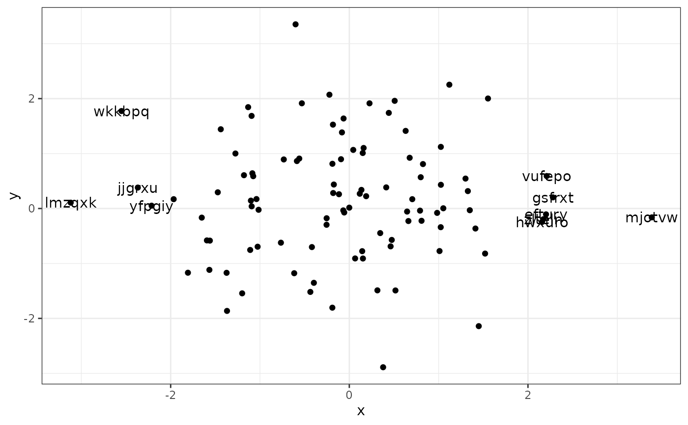
ggplot(data = d, aes(x, y, label = lab)) +
geom_point() +
stat_dens1d_labels()
 ggrepel.installed <- requireNamespace("ggrepel", quietly = TRUE)
if (ggrepel.installed) {
library(ggrepel)
# using defaults
ggplot(data = d, aes(x, y, label = lab)) +
geom_point() +
stat_dens1d_labels(geom = "text_repel")
# if no mapping to label is found, it is set row names
ggplot(data = d, aes(x, y)) +
geom_point() +
stat_dens1d_labels(geom = "text_repel")
ggplot(data = d, aes(x, y)) +
geom_point() +
stat_dens1d_labels(geom = "text_repel", pool.along = "none")
ggplot(data = d, aes(x, y)) +
geom_point() +
stat_dens1d_labels(geom = "text_repel",
keep.number = c(0, 10), pool.along = "none")
ggplot(data = d, aes(x, y)) +
geom_point() +
stat_dens1d_labels(geom = "text_repel",
keep.fraction = c(0, 0.2), pool.along = "none")
# using defaults, along y-axis
ggplot(data = d, aes(x, y, label = lab)) +
geom_point() +
stat_dens1d_labels(orientation = "y", geom = "text_repel")
# example labelling with coordiantes
ggplot(data = d, aes(x, y, label = sprintf("x = %.2f\ny = %.2f", x, y))) +
geom_point() +
stat_dens1d_filter(colour = "red") +
stat_dens1d_labels(geom = "text_repel", colour = "red", size = 3)
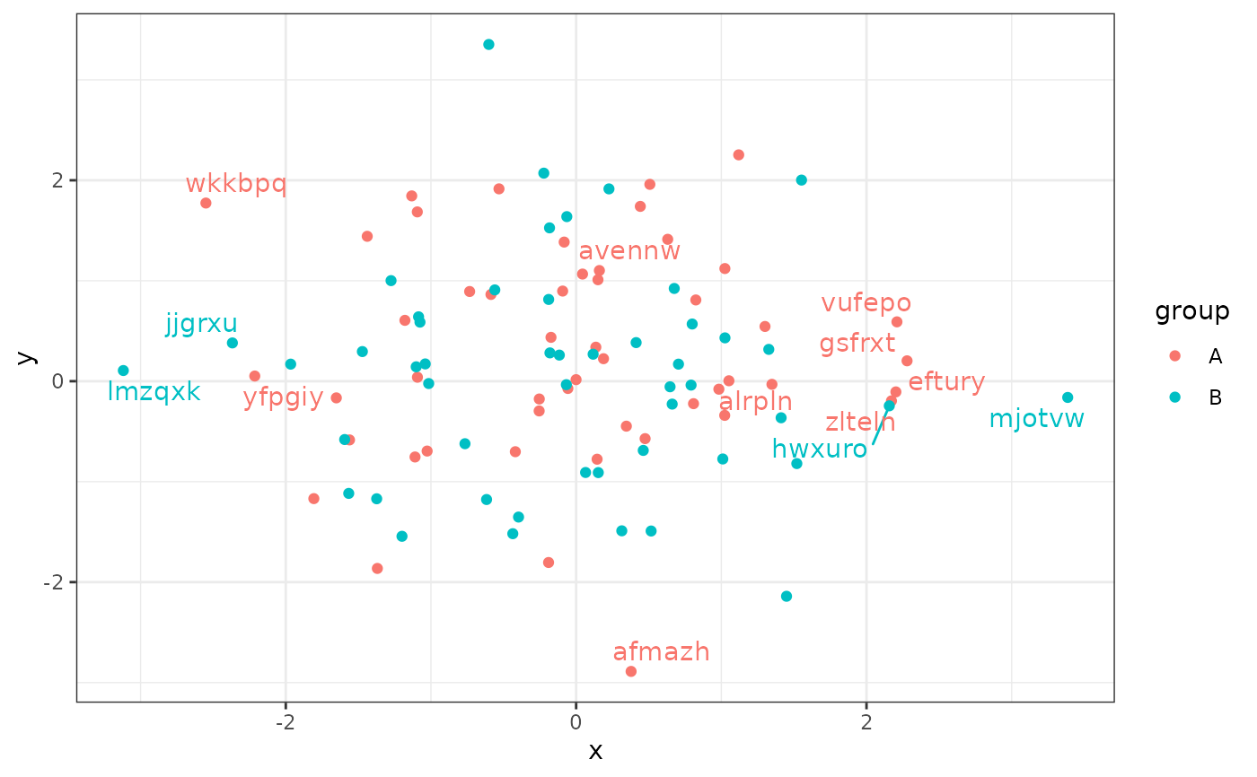
ggplot(data = d, aes(x, y, label = lab, colour = group)) +
geom_point() +
stat_dens1d_labels(geom = "text_repel")
ggplot(data = d, aes(x, y, label = lab, colour = group)) +
geom_point() +
stat_dens1d_labels(geom = "text_repel", label.fill = NA)
# we keep labels starting with "a" across the whole plot, but all in sparse
# regions. To achieve this we pass as argument to label.fill a fucntion
# instead of a character string.
label.fun <- function(x) {ifelse(grepl("^a", x), x, "")}
ggplot(data = d, aes(x, y, label = lab, colour = group)) +
geom_point() +
stat_dens1d_labels(geom = "text_repel", label.fill = label.fun)
}
ggrepel.installed <- requireNamespace("ggrepel", quietly = TRUE)
if (ggrepel.installed) {
library(ggrepel)
# using defaults
ggplot(data = d, aes(x, y, label = lab)) +
geom_point() +
stat_dens1d_labels(geom = "text_repel")
# if no mapping to label is found, it is set row names
ggplot(data = d, aes(x, y)) +
geom_point() +
stat_dens1d_labels(geom = "text_repel")
ggplot(data = d, aes(x, y)) +
geom_point() +
stat_dens1d_labels(geom = "text_repel", pool.along = "none")
ggplot(data = d, aes(x, y)) +
geom_point() +
stat_dens1d_labels(geom = "text_repel",
keep.number = c(0, 10), pool.along = "none")
ggplot(data = d, aes(x, y)) +
geom_point() +
stat_dens1d_labels(geom = "text_repel",
keep.fraction = c(0, 0.2), pool.along = "none")
# using defaults, along y-axis
ggplot(data = d, aes(x, y, label = lab)) +
geom_point() +
stat_dens1d_labels(orientation = "y", geom = "text_repel")
# example labelling with coordiantes
ggplot(data = d, aes(x, y, label = sprintf("x = %.2f\ny = %.2f", x, y))) +
geom_point() +
stat_dens1d_filter(colour = "red") +
stat_dens1d_labels(geom = "text_repel", colour = "red", size = 3)
ggplot(data = d, aes(x, y, label = lab, colour = group)) +
geom_point() +
stat_dens1d_labels(geom = "text_repel")
ggplot(data = d, aes(x, y, label = lab, colour = group)) +
geom_point() +
stat_dens1d_labels(geom = "text_repel", label.fill = NA)
# we keep labels starting with "a" across the whole plot, but all in sparse
# regions. To achieve this we pass as argument to label.fill a fucntion
# instead of a character string.
label.fun <- function(x) {ifelse(grepl("^a", x), x, "")}
ggplot(data = d, aes(x, y, label = lab, colour = group)) +
geom_point() +
stat_dens1d_labels(geom = "text_repel", label.fill = label.fun)
}
 # Using geom_debug() we can see that all 100 rows in \code{d} are
# returned. But only those labelled in the previous example still contain
# the original labels.
gginnards.installed <- requireNamespace("gginnards", quietly = TRUE)
if (gginnards.installed) {
library(gginnards)
ggplot(data = d, aes(x, y, label = lab)) +
geom_point() +
stat_dens1d_labels(geom = "debug")
ggplot(data = d, aes(x, y, label = lab)) +
geom_point() +
stat_dens1d_labels(geom = "debug", return.density = TRUE)
ggplot(data = d, aes(x, y, label = lab)) +
geom_point() +
stat_dens1d_labels(geom = "debug", label.fill = NULL, return.density = TRUE)
ggplot(data = d, aes(x, y, label = lab)) +
geom_point() +
stat_dens1d_labels(geom = "debug", label.fill = NA, return.density = TRUE)
ggplot(data = d, aes(x, y, label = lab)) +
geom_point() +
stat_dens1d_labels(geom = "debug", label.fill = FALSE, return.density = TRUE)
}
# Using geom_debug() we can see that all 100 rows in \code{d} are
# returned. But only those labelled in the previous example still contain
# the original labels.
gginnards.installed <- requireNamespace("gginnards", quietly = TRUE)
if (gginnards.installed) {
library(gginnards)
ggplot(data = d, aes(x, y, label = lab)) +
geom_point() +
stat_dens1d_labels(geom = "debug")
ggplot(data = d, aes(x, y, label = lab)) +
geom_point() +
stat_dens1d_labels(geom = "debug", return.density = TRUE)
ggplot(data = d, aes(x, y, label = lab)) +
geom_point() +
stat_dens1d_labels(geom = "debug", label.fill = NULL, return.density = TRUE)
ggplot(data = d, aes(x, y, label = lab)) +
geom_point() +
stat_dens1d_labels(geom = "debug", label.fill = NA, return.density = TRUE)
ggplot(data = d, aes(x, y, label = lab)) +
geom_point() +
stat_dens1d_labels(geom = "debug", label.fill = FALSE, return.density = TRUE)
}
 #> [1] "PANEL 1; group(s) -1; 'draw_function()' input 'data' (head):"
#> x y label PANEL group keep.obs density xintercept
#> 1 -1.02635566 -0.69517901 nkgqzv 1 -1 FALSE 0.23112677 0
#> 2 -1.10971271 -0.75422461 jkyqdg 1 -1 FALSE 0.22411433 0
#> 3 0.15034000 1.01021050 wznwfw 1 -1 FALSE 0.33020607 0
#> 4 -1.36919389 -1.86359713 mcrzfu 1 -1 FALSE 0.19529293 0
#> 5 -2.21355086 0.05160697 yfpgiy 1 -1 TRUE 0.06816381 0
#> 6 -0.08241679 1.38505284 bsyvwq 1 -1 FALSE 0.32495157 0
#> orientation
#> 1 x
#> 2 x
#> 3 x
#> 4 x
#> 5 x
#> 6 x
#> [1] "PANEL 1; group(s) -1; 'draw_function()' input 'data' (head):"
#> x y label PANEL group keep.obs density xintercept
#> 1 -1.02635566 -0.69517901 nkgqzv 1 -1 FALSE 0.23112677 0
#> 2 -1.10971271 -0.75422461 jkyqdg 1 -1 FALSE 0.22411433 0
#> 3 0.15034000 1.01021050 wznwfw 1 -1 FALSE 0.33020607 0
#> 4 -1.36919389 -1.86359713 mcrzfu 1 -1 FALSE 0.19529293 0
#> 5 -2.21355086 0.05160697 yfpgiy 1 -1 TRUE 0.06816381 0
#> 6 -0.08241679 1.38505284 bsyvwq 1 -1 FALSE 0.32495157 0
#> orientation
#> 1 x
#> 2 x
#> 3 x
#> 4 x
#> 5 x
#> 6 x