Support Vector Machines
svm.Rdsvm is used to train a support vector machine. It can be used to carry
out general regression and classification (of nu and epsilon-type), as
well as density-estimation. A formula interface is provided.
Usage
# S3 method for class 'formula'
svm(formula, data = NULL, ..., subset, na.action =
na.omit, scale = TRUE)
# Default S3 method
svm(x, y = NULL, scale = TRUE, type = NULL, kernel =
"radial", degree = 3, gamma = if (is.vector(x)) 1 else 1 / ncol(x),
coef0 = 0, cost = 1, nu = 0.5,
class.weights = NULL, cachesize = 40, tolerance = 0.001, epsilon = 0.1,
shrinking = TRUE, cross = 0, probability = FALSE, fitted = TRUE,
..., subset, na.action = na.omit)
Arguments
- formula
a symbolic description of the model to be fit.
- data
an optional data frame containing the variables in the model. By default the variables are taken from the environment which ‘svm’ is called from.
- x
a data matrix, a vector, or a sparse matrix (object of class
Matrixprovided by the Matrix package, or of classmatrix.csrprovided by the SparseM package, or of classsimple_triplet_matrixprovided by the slam package).- y
a response vector with one label for each row/component of
x. Can be either a factor (for classification tasks) or a numeric vector (for regression).- scale
A logical vector indicating the variables to be scaled. If
scaleis of length 1, the value is recycled as many times as needed. Per default, data are scaled internally (bothxandyvariables) to zero mean and unit variance. The center and scale values are returned and used for later predictions.- type
svmcan be used as a classification machine, as a regression machine, or for novelty detection. Depending of whetheryis a factor or not, the default setting fortypeisC-classificationoreps-regression, respectively, but may be overwritten by setting an explicit value.
Valid options are:C-classificationnu-classificationone-classification(for novelty detection)eps-regressionnu-regression
- kernel
the kernel used in training and predicting. You might consider changing some of the following parameters, depending on the kernel type.
- linear:
\(u'v\)
- polynomial:
\((\gamma u'v + coef0)^{degree}\)
- radial basis:
\(e^(-\gamma |u-v|^2)\)
- sigmoid:
\(tanh(\gamma u'v + coef0)\)
- degree
parameter needed for kernel of type
polynomial(default: 3)- gamma
parameter needed for all kernels except
linear(default: 1/(data dimension))- coef0
parameter needed for kernels of type
polynomialandsigmoid(default: 0)- cost
cost of constraints violation (default: 1)—it is the ‘C’-constant of the regularization term in the Lagrange formulation.
- nu
parameter needed for
nu-classification,nu-regression, andone-classification- class.weights
a named vector of weights for the different classes, used for asymmetric class sizes. Not all factor levels have to be supplied (default weight: 1). All components have to be named. Specifying
"inverse"will choose the weights inversely proportional to the class distribution.- cachesize
cache memory in MB (default 40)
- tolerance
tolerance of termination criterion (default: 0.001)
- epsilon
epsilon in the insensitive-loss function (default: 0.1)
- shrinking
option whether to use the shrinking-heuristics (default:
TRUE)- cross
if a integer value k>0 is specified, a k-fold cross validation on the training data is performed to assess the quality of the model: the accuracy rate for classification and the Mean Squared Error for regression
- fitted
logical indicating whether the fitted values should be computed and included in the model or not (default:
TRUE)- probability
logical indicating whether the model should allow for probability predictions.
- ...
additional parameters for the low level fitting function
svm.default- subset
An index vector specifying the cases to be used in the training sample. (NOTE: If given, this argument must be named.)
- na.action
A function to specify the action to be taken if
NAs are found. The default action isna.omit, which leads to rejection of cases with missing values on any required variable. An alternative isna.fail, which causes an error ifNAcases are found. (NOTE: If given, this argument must be named.)
Value
An object of class "svm" containing the fitted model, including:
- SV
The resulting support vectors (possibly scaled).
- index
The index of the resulting support vectors in the data matrix. Note that this index refers to the preprocessed data (after the possible effect of
na.omitandsubset)- coefs
The corresponding coefficients times the training labels.
- rho
The negative intercept.
- sigma
In case of a probabilistic regression model, the scale parameter of the hypothesized (zero-mean) laplace distribution estimated by maximum likelihood.
- probA, probB
numeric vectors of length k(k-1)/2, k number of classes, containing the parameters of the logistic distributions fitted to the decision values of the binary classifiers (1 / (1 + exp(a x + b))).
Details
For multiclass-classification with k levels, k>2, libsvm uses the
‘one-against-one’-approach, in which k(k-1)/2 binary classifiers are
trained; the appropriate class is found by a voting scheme.
libsvm internally uses a sparse data representation, which is
also high-level supported by the package SparseM.
If the predictor variables include factors, the formula interface must be used to get a correct model matrix.
plot.svm allows a simple graphical
visualization of classification models.
The probability model for classification fits a logistic distribution using maximum likelihood to the decision values of all binary classifiers, and computes the a-posteriori class probabilities for the multi-class problem using quadratic optimization. The probabilistic regression model assumes (zero-mean) laplace-distributed errors for the predictions, and estimates the scale parameter using maximum likelihood.
For linear kernel, the coefficients of the regression/decision hyperplane
can be extracted using the coef method (see examples).
Note
Data are scaled internally, usually yielding better results.
Parameters of SVM-models usually must be tuned to yield sensible results!
References
Chang, Chih-Chung and Lin, Chih-Jen:
LIBSVM: a library for Support Vector Machines
https://www.csie.ntu.edu.tw/~cjlin/libsvm/Exact formulations of models, algorithms, etc. can be found in the document:
Chang, Chih-Chung and Lin, Chih-Jen:
LIBSVM: a library for Support Vector Machines
https://www.csie.ntu.edu.tw/~cjlin/papers/libsvm.ps.gzMore implementation details and speed benchmarks can be found on: Rong-En Fan and Pai-Hsune Chen and Chih-Jen Lin:
Working Set Selection Using the Second Order Information for Training SVM
https://www.csie.ntu.edu.tw/~cjlin/papers/quadworkset.pdf
Author
David Meyer (based on C/C++-code by Chih-Chung Chang and Chih-Jen Lin)
David.Meyer@R-project.org
See also
predict.svm
plot.svm
tune.svm
matrix.csr (in package SparseM)
Examples
data(iris)
attach(iris)
#> The following objects are masked from iris (pos = 4):
#>
#> Petal.Length, Petal.Width, Sepal.Length, Sepal.Width, Species
## classification mode
# default with factor response:
model <- svm(Species ~ ., data = iris)
# alternatively the traditional interface:
x <- subset(iris, select = -Species)
y <- Species
model <- svm(x, y)
print(model)
#>
#> Call:
#> svm.default(x = x, y = y)
#>
#>
#> Parameters:
#> SVM-Type: C-classification
#> SVM-Kernel: radial
#> cost: 1
#>
#> Number of Support Vectors: 51
#>
summary(model)
#>
#> Call:
#> svm.default(x = x, y = y)
#>
#>
#> Parameters:
#> SVM-Type: C-classification
#> SVM-Kernel: radial
#> cost: 1
#>
#> Number of Support Vectors: 51
#>
#> ( 8 22 21 )
#>
#>
#> Number of Classes: 3
#>
#> Levels:
#> setosa versicolor virginica
#>
#>
#>
# test with train data
pred <- predict(model, x)
# (same as:)
pred <- fitted(model)
# Check accuracy:
table(pred, y)
#> y
#> pred setosa versicolor virginica
#> setosa 50 0 0
#> versicolor 0 48 2
#> virginica 0 2 48
# compute decision values and probabilities:
pred <- predict(model, x, decision.values = TRUE)
attr(pred, "decision.values")[1:4,]
#> setosa/versicolor setosa/virginica versicolor/virginica
#> 1 1.196152 1.091757 0.6708810
#> 2 1.064621 1.056185 0.8483518
#> 3 1.180842 1.074542 0.6439798
#> 4 1.110699 1.053012 0.6782041
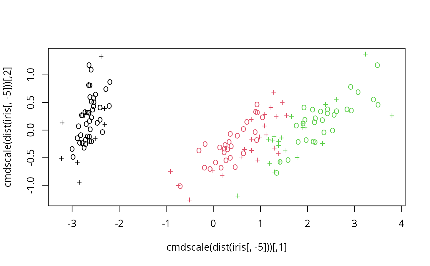
# visualize (classes by color, SV by crosses):
plot(cmdscale(dist(iris[,-5])),
col = as.integer(iris[,5]),
pch = c("o","+")[1:150 %in% model$index + 1])
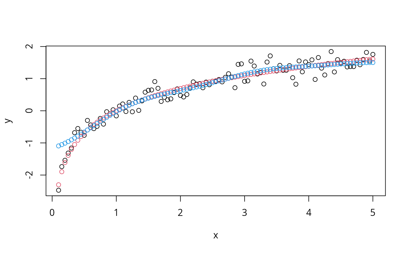
 ## try regression mode on two dimensions
# create data
x <- seq(0.1, 5, by = 0.05)
y <- log(x) + rnorm(x, sd = 0.2)
# estimate model and predict input values
m <- svm(x, y)
new <- predict(m, x)
# visualize
plot(x, y)
points(x, log(x), col = 2)
points(x, new, col = 4)
## try regression mode on two dimensions
# create data
x <- seq(0.1, 5, by = 0.05)
y <- log(x) + rnorm(x, sd = 0.2)
# estimate model and predict input values
m <- svm(x, y)
new <- predict(m, x)
# visualize
plot(x, y)
points(x, log(x), col = 2)
points(x, new, col = 4)
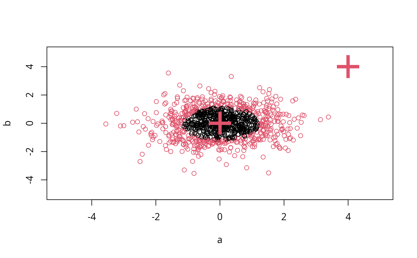
 ## density-estimation
# create 2-dim. normal with rho=0:
X <- data.frame(a = rnorm(1000), b = rnorm(1000))
attach(X)
#> The following objects are masked from X (pos = 4):
#>
#> a, b
# traditional way:
m <- svm(X, gamma = 0.1)
# formula interface:
m <- svm(~., data = X, gamma = 0.1)
# or:
m <- svm(~ a + b, gamma = 0.1)
# test:
newdata <- data.frame(a = c(0, 4), b = c(0, 4))
predict (m, newdata)
#> 1 2
#> TRUE FALSE
# visualize:
plot(X, col = 1:1000 %in% m$index + 1, xlim = c(-5,5), ylim=c(-5,5))
points(newdata, pch = "+", col = 2, cex = 5)
## density-estimation
# create 2-dim. normal with rho=0:
X <- data.frame(a = rnorm(1000), b = rnorm(1000))
attach(X)
#> The following objects are masked from X (pos = 4):
#>
#> a, b
# traditional way:
m <- svm(X, gamma = 0.1)
# formula interface:
m <- svm(~., data = X, gamma = 0.1)
# or:
m <- svm(~ a + b, gamma = 0.1)
# test:
newdata <- data.frame(a = c(0, 4), b = c(0, 4))
predict (m, newdata)
#> 1 2
#> TRUE FALSE
# visualize:
plot(X, col = 1:1000 %in% m$index + 1, xlim = c(-5,5), ylim=c(-5,5))
points(newdata, pch = "+", col = 2, cex = 5)
 ## weights: (example not particularly sensible)
i2 <- iris
levels(i2$Species)[3] <- "versicolor"
summary(i2$Species)
#> setosa versicolor
#> 50 100
wts <- 100 / table(i2$Species)
wts
#>
#> setosa versicolor
#> 2 1
m <- svm(Species ~ ., data = i2, class.weights = wts)
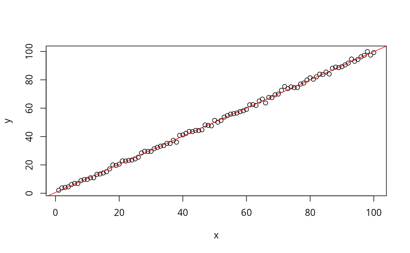
## extract coefficients for linear kernel
# a. regression
x <- 1:100
y <- x + rnorm(100)
m <- svm(y ~ x, scale = FALSE, kernel = "linear")
coef(m)
#> (Intercept) x
#> 0.5649707 0.9926688
plot(y ~ x)
abline(m, col = "red")
## weights: (example not particularly sensible)
i2 <- iris
levels(i2$Species)[3] <- "versicolor"
summary(i2$Species)
#> setosa versicolor
#> 50 100
wts <- 100 / table(i2$Species)
wts
#>
#> setosa versicolor
#> 2 1
m <- svm(Species ~ ., data = i2, class.weights = wts)
## extract coefficients for linear kernel
# a. regression
x <- 1:100
y <- x + rnorm(100)
m <- svm(y ~ x, scale = FALSE, kernel = "linear")
coef(m)
#> (Intercept) x
#> 0.5649707 0.9926688
plot(y ~ x)
abline(m, col = "red")
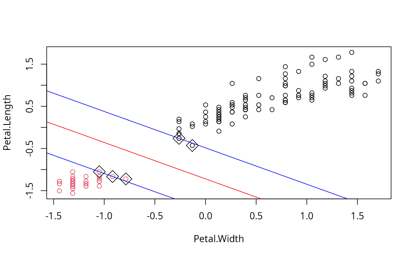
 # b. classification
# transform iris data to binary problem, and scale data
setosa <- as.factor(iris$Species == "setosa")
iris2 = scale(iris[,-5])
# fit binary C-classification model
m <- svm(setosa ~ Petal.Width + Petal.Length,
data = iris2, kernel = "linear")
# plot data and separating hyperplane
plot(Petal.Length ~ Petal.Width, data = iris2, col = setosa)
(cf <- coef(m))
#> (Intercept) Petal.Width Petal.Length
#> -1.658953 -1.172523 -1.358030
abline(-cf[1]/cf[3], -cf[2]/cf[3], col = "red")
# plot margin and mark support vectors
abline(-(cf[1] + 1)/cf[3], -cf[2]/cf[3], col = "blue")
abline(-(cf[1] - 1)/cf[3], -cf[2]/cf[3], col = "blue")
points(m$SV, pch = 5, cex = 2)
# b. classification
# transform iris data to binary problem, and scale data
setosa <- as.factor(iris$Species == "setosa")
iris2 = scale(iris[,-5])
# fit binary C-classification model
m <- svm(setosa ~ Petal.Width + Petal.Length,
data = iris2, kernel = "linear")
# plot data and separating hyperplane
plot(Petal.Length ~ Petal.Width, data = iris2, col = setosa)
(cf <- coef(m))
#> (Intercept) Petal.Width Petal.Length
#> -1.658953 -1.172523 -1.358030
abline(-cf[1]/cf[3], -cf[2]/cf[3], col = "red")
# plot margin and mark support vectors
abline(-(cf[1] + 1)/cf[3], -cf[2]/cf[3], col = "blue")
abline(-(cf[1] - 1)/cf[3], -cf[2]/cf[3], col = "blue")
points(m$SV, pch = 5, cex = 2)