Predict Method for Support Vector Machines

This function predicts values based upon a model trained by svm.

Usage

# S3 method for class 'svm'
predict(object, newdata, decision.values = FALSE,
probability = FALSE, ..., na.action = na.omit)

Arguments

object: Object of class "svm", created by svm.
newdata: An object containing the new input data: either a matrix or a sparse matrix (object of class Matrix provided by the Matrix package, or of class matrix.csr provided by the SparseM package, or of class simple_triplet_matrix provided by the slam package). A vector will be transformed to a n x 1 matrix.
decision.values: Logical controlling whether the decision values of all binary classifiers computed in multiclass classification shall be computed and returned.
probability: Logical indicating whether class probabilities should be computed and returned. Only possible if the model was fitted with the probability option enabled.
na.action: A function to specify the action to be taken if ‘NA’s are found. The default action is na.omit, which leads to rejection of cases with missing values on any required variable. An alternative is na.fail, which causes an error if NA cases are found. (NOTE: If given, this argument must be named.)
...: Currently not used.

Value

A vector of predicted values (for classification: a vector of labels, for density estimation: a logical vector). If decision.value is TRUE, the vector gets a "decision.values" attribute containing a n x c matrix (n number of predicted values, c number of classifiers) of all c binary classifiers' decision values. There are k * (k - 1) / 2 classifiers (k number of classes). The colnames of the matrix indicate the labels of the two classes. If probability is TRUE, the vector gets a "probabilities" attribute containing a n x k matrix (n number of predicted values, k number of classes) of the class probabilities.

Note

If the training set was scaled by svm (done by default), the new data is scaled accordingly using scale and center of the training data.

Author

David Meyer (based on C++-code by Chih-Chung Chang and Chih-Jen Lin)
David.Meyer@R-project.org

Examples

data(iris)
attach(iris)

## classification mode
# default with factor response:
model <- svm(Species ~ ., data = iris)

# alternatively the traditional interface:
x <- subset(iris, select = -Species)
y <- Species
model <- svm(x, y, probability = TRUE) 

print(model)
#> 
#> Call:
#> svm.default(x = x, y = y, probability = TRUE)
#> 
#> 
#> Parameters:
#>    SVM-Type:  C-classification 
#>  SVM-Kernel:  radial 
#>        cost:  1 
#> 
#> Number of Support Vectors:  51
#> 
summary(model)
#> 
#> Call:
#> svm.default(x = x, y = y, probability = TRUE)
#> 
#> 
#> Parameters:
#>    SVM-Type:  C-classification 
#>  SVM-Kernel:  radial 
#>        cost:  1 
#> 
#> Number of Support Vectors:  51
#> 
#>  ( 8 22 21 )
#> 
#> 
#> Number of Classes:  3 
#> 
#> Levels: 
#>  setosa versicolor virginica
#> 
#> 
#> 

# test with train data
pred <- predict(model, x)
# (same as:)
pred <- fitted(model)

# compute decision values and probabilites
pred <- predict(model, x, decision.values = TRUE, probability = TRUE)
attr(pred, "decision.values")[1:4,]
#>   setosa/versicolor setosa/virginica versicolor/virginica
#> 1          1.196152         1.091757            0.6708810
#> 2          1.064621         1.056185            0.8483518
#> 3          1.180842         1.074542            0.6439798
#> 4          1.110699         1.053012            0.6782041
attr(pred, "probabilities")[1:4,]
#>      setosa versicolor   virginica
#> 1 0.9799440 0.01105443 0.009001534
#> 2 0.9726238 0.01772298 0.009653187
#> 3 0.9786104 0.01166303 0.009726537
#> 4 0.9745697 0.01497637 0.010453974

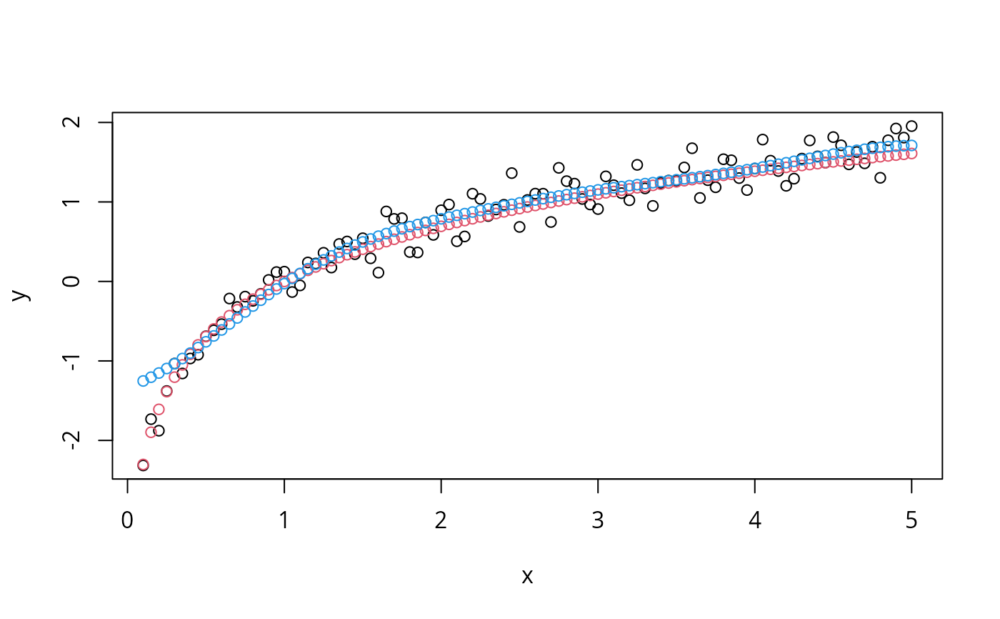
## try regression mode on two dimensions

# create data
x <- seq(0.1, 5, by = 0.05)
y <- log(x) + rnorm(x, sd = 0.2)

# estimate model and predict input values
m   <- svm(x, y)
new <- predict(m, x)

# visualize
plot   (x, y)
points (x, log(x), col = 2)
points (x, new, col = 4)


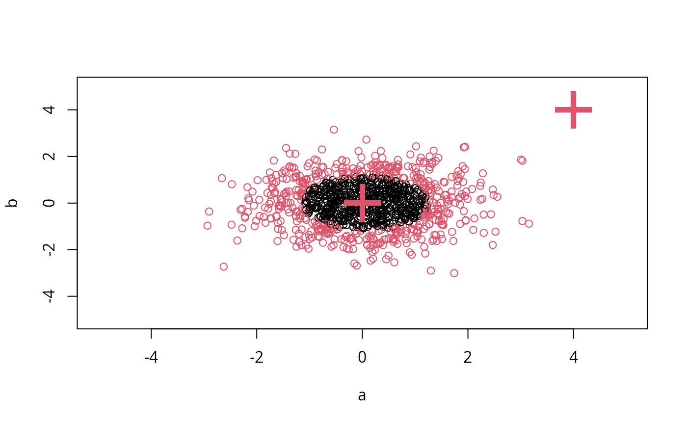
## density-estimation

# create 2-dim. normal with rho=0:
X <- data.frame(a = rnorm(1000), b = rnorm(1000))
attach(X)

# traditional way:
m <- svm(X, gamma = 0.1)

# formula interface:
m <- svm(~., data = X, gamma = 0.1)
# or:
m <- svm(~ a + b, gamma = 0.1)

# test:
newdata <- data.frame(a = c(0, 4), b = c(0, 4))
predict (m, newdata)
#>     1     2 
#>  TRUE FALSE 

# visualize:
plot(X, col = 1:1000 %in% m$index + 1, xlim = c(-5,5), ylim=c(-5,5))
points(newdata, pch = "+", col = 2, cex = 5)