Regression Leverage Plots

These functions display a generalization, due to Sall (1990) and Cook and Weisberg (1991), of added-variable plots to multiple-df terms in a linear model. When a term has just 1 df, the leverage plot is a rescaled version of the usual added-variable (partial-regression) plot.

Usage

leveragePlots(model, terms = ~., layout = NULL, ask, 
    main, ...)

leveragePlot(model, ...)

# S3 method for class 'lm'
leveragePlot(model, term.name,
    id=TRUE, col=carPalette()[1], col.lines=carPalette()[2], lwd=2, 
    xlab, ylab, main="Leverage Plot", grid=TRUE, ...)

# S3 method for class 'glm'
leveragePlot(model, ...)

Arguments

model: model object produced by lm
terms: A one-sided formula that specifies a subset of the numeric regressors, factors and interactions. One added-variable plot is drawn for each term, either a main effect or an interactions. The default ~. is to plot against all terms in the model. For example, the specification terms = ~ . - X3 would plot against all predictors except for X3. If this argument is a quoted name of one of the predictors, the added-variable plot is drawn for that predictor only. The plots for main effects with interactions present violate the marginality principle and may not be easily interpreted.
layout: If set to a value like c(1, 1) or c(4, 3), the layout of the graph will have this many rows and columns. If not set, the program will select an appropriate layout. If the number of graphs exceed nine, you must select the layout yourself, or you will get a maximum of nine per page. If layout=NA, the function does not set the layout and the user can use the par function to control the layout, for example to have plots from two models in the same graphics window.
ask: if TRUE, a menu is provided in the R Console for the user to select the term(s) to plot.
xlab, ylab: axis labels; if missing, labels will be supplied.
main: title for plot; if missing, a title will be supplied.
...: arguments passed down to method functions.
term.name: Quoted name of term in the model to be plotted; this argument is omitted for leveragePlots.
id: controls point identification; if FALSE, no points are identified; can be a list of named arguments to the showLabels function; TRUE, the default, is equivalent to list(method=list(abs(residuals(model, type="pearson")), "x"), n=2, cex=1, col=carPalette()[1], location="lr"), which identifies the 2 points with the largest residuals and the 2 points with the greatest partial leverage.
col: color(s) of points
col.lines: color of the fitted line
lwd: line width; default is 2 (see par).
grid: If TRUE, the default, a light-gray background grid is put on the graph

Details

The function intended for direct use is leveragePlots.

The model can contain factors and interactions. A leverage plot can be drawn for each term in the model, including the constant.

leveragePlot.glm is a dummy function, which generates an error message.

Value

NULL. These functions are used for their side effect: producing plots.

References

Cook, R. D. and Weisberg, S. (1991). Added Variable Plots in Linear Regression. In Stahel, W. and Weisberg, S. (eds.), Directions in Robust Statistics and Diagnostics. Springer, 47-60.

Fox, J. (2016) Applied Regression Analysis and Generalized Linear Models, Third Edition. Sage.

Fox, J. and Weisberg, S. (2019) An R Companion to Applied Regression, Third Edition, Sage.

Sall, J. (1990) Leverage plots for general linear hypotheses. American Statistician 44, 308–315.

Author

John Fox jfox@mcmaster.ca

Examples

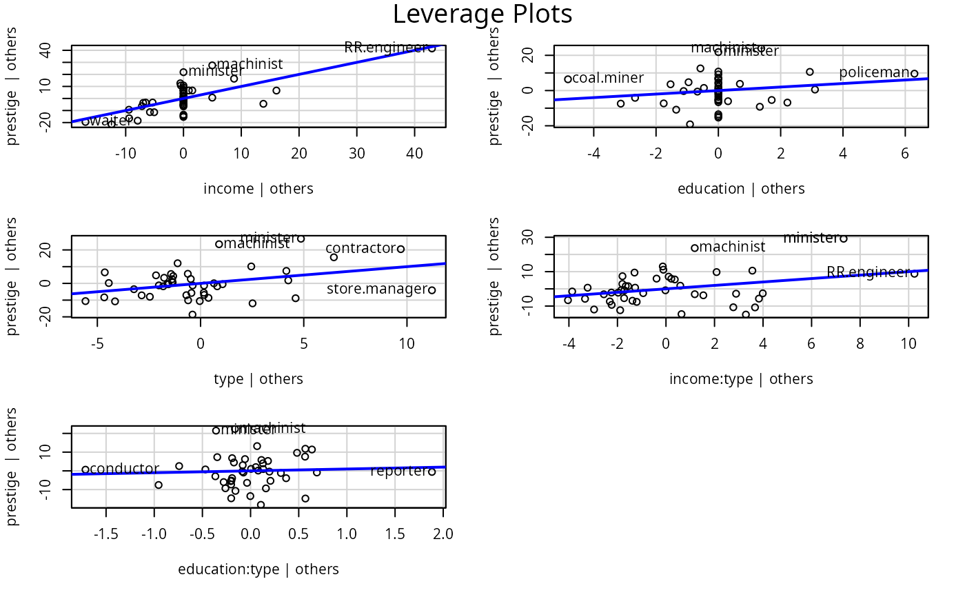
leveragePlots(lm(prestige~(income+education)*type, data=Duncan))