Choose a Predictor Transformation Visually or Numerically

invTranPlot draws a two-dimensional scatterplot of \(Y\) versus \(X\), along with the OLS fit from the regression of \(Y\) on \((X^{\lambda}-1)/\lambda\). invTranEstimate finds the nonlinear least squares estimate of \(\lambda\) and its standard error.

Usage

invTranPlot(x, ...)

# S3 method for class 'formula'
invTranPlot(x, data, subset, na.action, id=FALSE, ...)

# Default S3 method
invTranPlot(x, y, lambda=c(-1, 0, 1), robust=FALSE, 
        lty.lines=rep(c("solid", "dashed", "dotdash", "longdash", "twodash"), 
        length=1 + length(lambda)), lwd.lines=2, 
        col=carPalette()[1], col.lines=carPalette(), 
        xlab=deparse(substitute(x)), ylab=deparse(substitute(y)),
        family="bcPower", optimal=TRUE, key="auto", id=FALSE,
        grid=TRUE, ...)

invTranEstimate(x, y, family="bcPower", confidence=0.95, robust=FALSE)

Arguments

x: The predictor variable, or a formula with a single response and a single predictor
y: The response variable
data: An optional data frame to get the data for the formula
subset: Optional, as in lm, select a subset of the cases
na.action: Optional, as in lm, the action for missing data
lambda: The powers used in the plot. The optimal power than minimizes the residual sum of squares is always added unless optimal is FALSE.
robust: If TRUE, then the estimated transformation is computed using Huber M-estimation with the MAD used to estimate scale and k=1.345. The default is FALSE.
family: The transformation family to use, "bcPower", "yjPower", or a user-defined family.
confidence: returns a profile likelihood confidence interval for the optimal transformation with this confidence level. If FALSE, or if robust=TRUE, no interval is returned.
optimal: Include the optimal value of lambda?
lty.lines: line types corresponding to the powers
lwd.lines: the width of the plotted lines, defaults to 2 times the standard
col: color(s) of the points in the plot. If you wish to distinguish points according to the levels of a factor, we recommend using symbols, specified with the pch argument, rather than colors.
col.lines: color of the fitted lines corresponding to the powers. The default is to use the colors returned by carPalette
key: The default is "auto", in which case a legend is added to the plot, either above the top marign or in the bottom right or top right corner. Set to NULL to suppress the legend.
xlab: Label for the horizontal axis.
ylab: Label for the vertical axis.
id: controls point identification; if FALSE (the default), no points are identified; can be a list of named arguments to the showLabels function; TRUE is equivalent to list(method=list(method="x", n=2, cex=1, col=carPalette()[1], location="lr"), which identifies the 2 points with the most extreme horizontal values — i.e., the response variable in the model.
...: Additional arguments passed to the plot method, such as pch.
grid: If TRUE, the default, a light-gray background grid is put on the graph

Value

invTranPlot plots a graph and returns a data frame with \(\lambda\) in the first column, and the residual sum of squares from the regression for that \(\lambda\) in the second column.

invTranEstimate returns a list with elements lambda for the estimate, se for its standard error, and RSS, the minimum value of the residual sum of squares.

References

Fox, J. and Weisberg, S. (2011) An R Companion to Applied Regression, Second Edition, Sage.

Prendergast, L. A., & Sheather, S. J. (2013) On sensitivity of inverse response plot estimation and the benefits of a robust estimation approach. Scandinavian Journal of Statistics, 40(2), 219-237.

Weisberg, S. (2014) Applied Linear Regression, Fourth Edition, Wiley, Chapter 7.

Author

Sanford Weisberg, sandy@umn.edu

Examples

with(UN, invTranPlot(ppgdp, infantMortality))

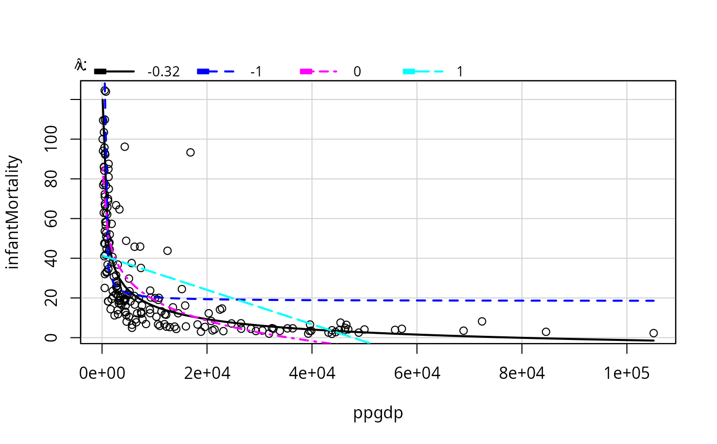#>       lambda       RSS
#> 1 -0.3208097  54816.14
#> 2 -1.0000000  83395.51
#> 3  0.0000000  62851.31
#> 4  1.0000000 120583.35
with(UN, invTranEstimate(ppgdp, infantMortality))
#> $lambda
#> [1] -0.3208097
#> 
#> $lowerCI
#> [1] -0.4034811
#> 
#> $upperCI
#> [1] -0.2386709
#>