Influence Index Plot

Provides index plots of influence and related diagnostics for a regression model.

Usage

infIndexPlot(model, ...)

influenceIndexPlot(model, ...)

# S3 method for class 'lm'
infIndexPlot(model, vars=c("Cook", "Studentized", "Bonf", "hat"),
    id=TRUE, grid=TRUE, main="Diagnostic Plots", ...)

# S3 method for class 'influence.merMod'
infIndexPlot(model,
    vars = c("dfbeta", "dfbetas", "var.cov.comps",
    "cookd"), id = TRUE, grid = TRUE, main = "Diagnostic Plots", ...)
# S3 method for class 'influence.lme'
infIndexPlot(model,
    vars = c("dfbeta", "dfbetas", "var.cov.comps",
    "cookd"), id = TRUE, grid = TRUE, main = "Diagnostic Plots", ...)

Arguments

model: A regression object of class lm, glm, or lmerMod, or an influence object for a lmer, glmer, or lme object (see influence.mixed.models). The "lmerMod" method calls the "lm" method and can take the same arguments.
vars: All the quantities listed in this argument are plotted. Use "Cook" for Cook's distances, "Studentized" for Studentized residuals, "Bonf" for Bonferroni p-values for an outlier test, and and "hat" for hat-values (or leverages) for a linear or generalized linear model, or "dfbeta", "dfbetas", "var.cov.comps", and "cookd" for an influence object derived from a mixed model. Capitalization is optional. All but "dfbeta" and "dfbetas" may be abbreviated by the first one or more letters.
main: main title for graph
id: a list of named values controlling point labelling. The default, TRUE, is equivalent to id=list(method="y", n=2, cex=1, col=carPalette()[1], location="lr"); FALSE suppresses point labelling. See showLabels for details.
grid: If TRUE, the default, a light-gray background grid is put on the graph.
...: Arguments passed to plot

Value

Used for its side effect of producing a graph. Produces index plots of diagnostic quantities.

References

Cook, R. D. and Weisberg, S. (1999) Applied Regression, Including Computing and Graphics. Wiley.

Fox, J. (2016) Applied Regression Analysis and Generalized Linear Models, Third Edition. Sage. Fox, J. and Weisberg, S. (2019) An R Companion to Applied Regression, Third Edition, Sage.

Weisberg, S. (2014) Applied Linear Regression, Fourth Edition, Wiley.

Author

Sanford Weisberg sandy@umn.edu and John Fox

Examples

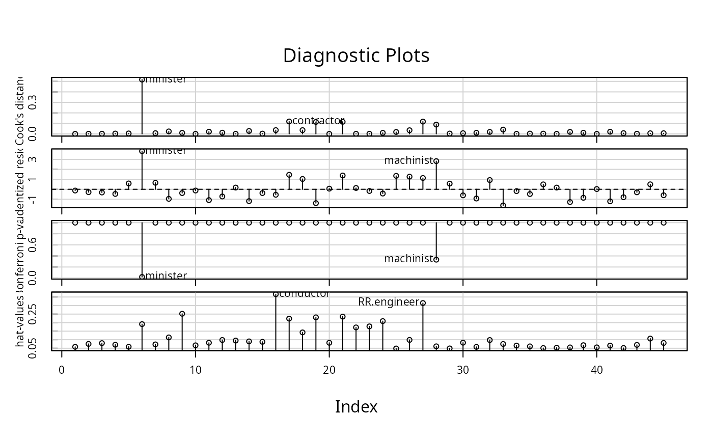
influenceIndexPlot(lm(prestige ~ income + education + type, Duncan))


if (FALSE)  # a little slow
  if (require(lme4)){
      print(fm1 <- lmer(Reaction ~ Days + (Days | Subject),
          sleepstudy)) # from ?lmer
      infIndexPlot(influence(fm1, "Subject"))
      infIndexPlot(influence(fm1))
      }
      
  if (require(lme4)){
      gm1 <- glmer(cbind(incidence, size - incidence) ~ period + (1 | herd),
          data = cbpp, family = binomial) # from ?glmer
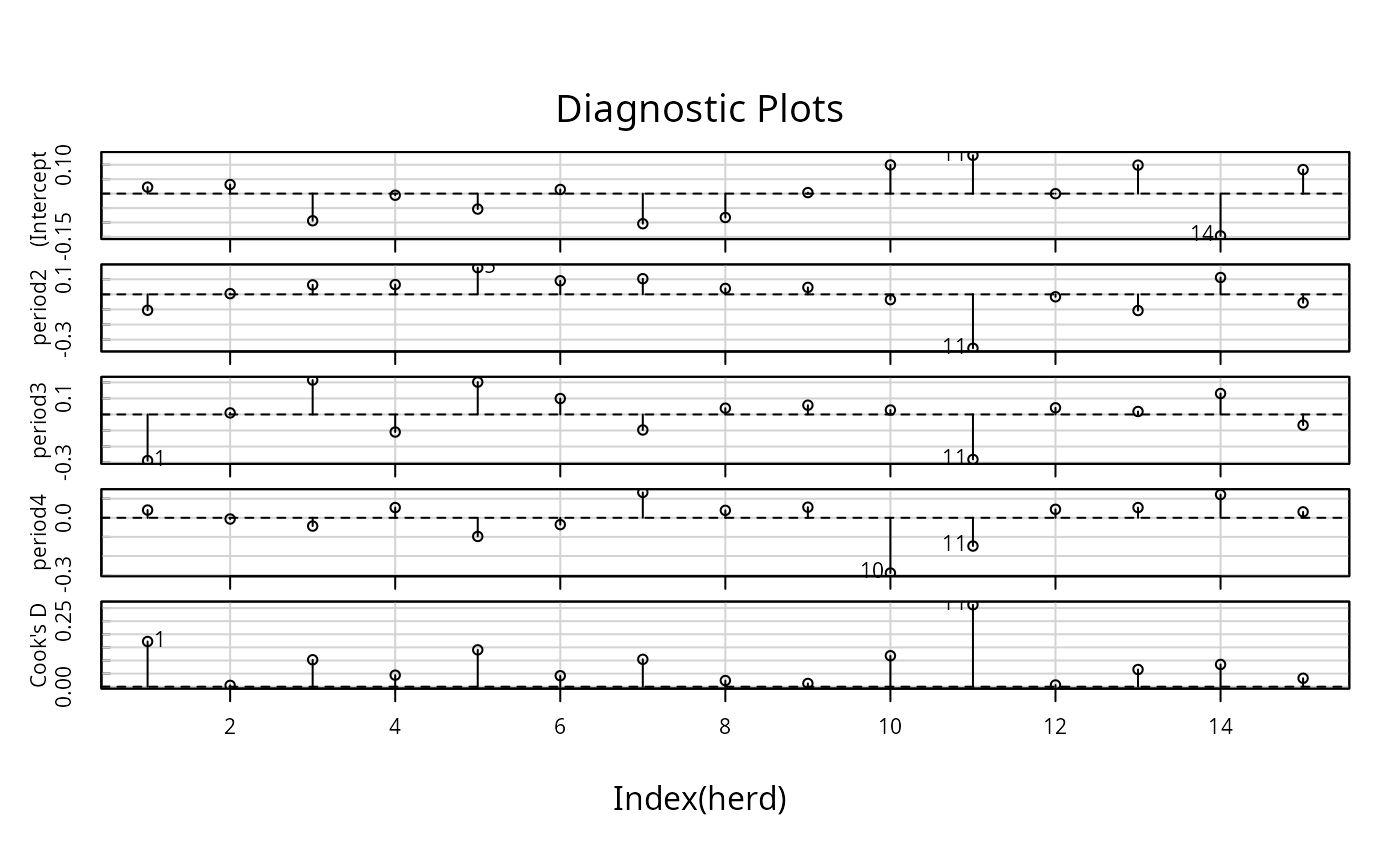
      infIndexPlot(influence(gm1, "herd", maxfun=100))
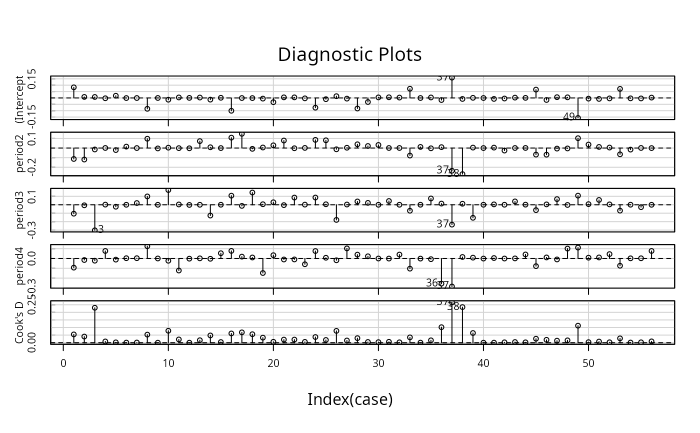
      infIndexPlot(influence(gm1, maxfun=100))
      gm1.11 <- update(gm1, subset = herd != 11) # check deleting herd 11
      compareCoefs(gm1, gm1.11)
      }
#> Loading required package: lme4
#> Loading required package: Matrix
#> 
#> Attaching package: ‘lme4’
#> The following object is masked from ‘package:rio’:
#> 
#>     factorize


#> Calls:
#> 1: glmer(formula = cbind(incidence, size - incidence) ~ period + (1 | herd),
#>    data = cbpp, family = binomial)
#> 2: glmer(formula = cbind(incidence, size - incidence) ~ period + (1 | herd),
#>    data = cbpp, family = binomial, subset = herd != 11)
#> 
#>             Model 1 Model 2
#> (Intercept)  -1.398  -1.271
#> SE            0.231   0.240
#>                            
#> period2      -0.992  -1.364
#> SE            0.303   0.343
#>                            
#> period3      -1.128  -1.399
#> SE            0.323   0.354
#>                            
#> period4      -1.580  -1.710
#> SE            0.422   0.453
#>                            
     # \dontrun{}