Attribute Plots

For all examples the movies data set contained in the package will be used.

library(UpSetR); library(ggplot2); library(grid); library(plyr)
movies <- read.csv( system.file("extdata", "movies.csv", package = "UpSetR"), header=T, sep=";" )

attribute.plots Parameter Breakdown

The attribute.plots parameter is broken down into 3 fields: gridrows, plots, and ncols

gridrows: specifies how much to expand the plot window to add room for attribute plots. The UpSetR plot is plotted on a 100 by 100 grid. So for example, if we set gridrows to 50, the new grid layout would be 150 by 100, setting aside 1/3 of the plot for the attribute plots.
plots: takes a list of paramters. These paramters include plot, x, y (if applicable), and queries.
plot: is a function that returns a ggplot
x: is the x aesthetic to be used in the ggplot (entered as string)
y: is the y aesthetic to be used in the ggplot (entered as string)
queries: indicates whether or not to overlay the plot with the queries present. If queries is TRUE, the attribute plot will be overlayed with data from the queries. If queries is FALSE, no query results will be plotted on the attribute plot.
ncols: specifies how the plots should be arranged in the gridrows space. If two attribute plots are entered and ncols is 1,then the plots will display one above the other. Alternatively, if two attribute plots are entered and ncols is 2, the attribute plots will be displayed side by side.

Additional: to add a legend of the queries, use query.legend = "bottom" (see Example 2).

Example 1: Built-In Attribute Histogram

Example of how to add built-in histogram attribute plot. If main.bar.color is not specified as black, elements contained in black intersection size bars will be represented as gray in attribute plots.

upset(movies, main.bar.color = "black", queries = list(list(query = intersects, params = list("Drama"), active = T)), attribute.plots = list(gridrows = 50, plots = list(list(plot = histogram, x = "ReleaseDate", queries = F), list(plot = histogram, x = "AvgRating", queries = T)), ncols = 2))

## Warning: `aes_string()` was deprecated in ggplot2 3.0.0.
## ℹ Please use tidy evaluation idioms with `aes()`.
## ℹ See also `vignette("ggplot2-in-packages")` for more information.
## ℹ The deprecated feature was likely used in the UpSetR package.
##   Please report the issue to the authors.
## This warning is displayed once every 8 hours.
## Call `lifecycle::last_lifecycle_warnings()` to see where this warning was
## generated.

## Warning in geom_point(data = pInterDat, aes_string(x = "x", y = "freq"), :
## Ignoring empty aesthetic: `colour`.

## Warning: Using `size` aesthetic for lines was deprecated in ggplot2 3.4.0.
## ℹ Please use `linewidth` instead.
## ℹ The deprecated feature was likely used in the UpSetR package.
##   Please report the issue to the authors.
## This warning is displayed once every 8 hours.
## Call `lifecycle::last_lifecycle_warnings()` to see where this warning was
## generated.

## Warning: The `size` argument of `element_line()` is deprecated as of ggplot2 3.4.0.
## ℹ Please use the `linewidth` argument instead.
## ℹ The deprecated feature was likely used in the UpSetR package.
##   Please report the issue to the authors.
## This warning is displayed once every 8 hours.
## Call `lifecycle::last_lifecycle_warnings()` to see where this warning was
## generated.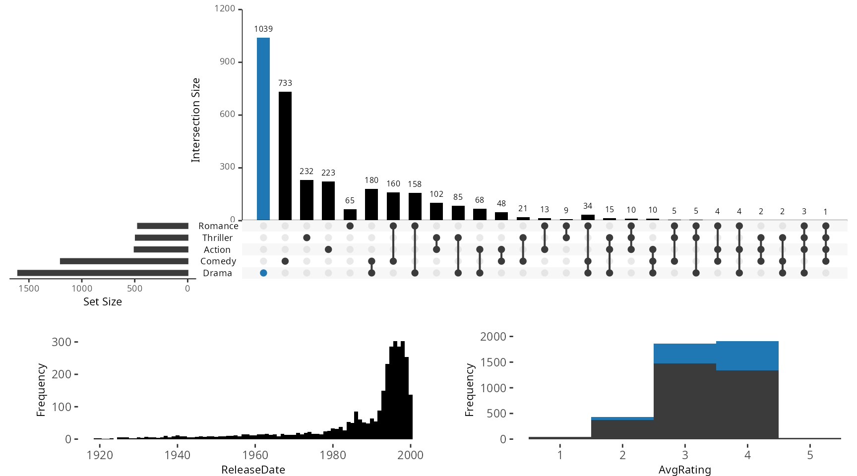

Example 2: Built-In Attribute Scatter Plot

Example of how to add built-in attribute scatter plot. If main.bar.color not specified as black, elements contained in black intersection size bars will be represented as gray in attribute plots.

notice the use of query.legend

upset(movies, main.bar.color = "black", queries = list(list(query = intersects, params = list("Drama"), color = "red", active = F), list(query = intersects, params = list("Action", "Drama"), active = T), list(query = intersects, params = list("Drama", "Comedy", "Action"), color = "orange", active = T)), attribute.plots = list(gridrows = 45, plots = list(list(plot = scatter_plot, x = "ReleaseDate", y = "AvgRating", queries = T), list(plot = scatter_plot, x = "AvgRating", y = "Watches", queries = F)), ncols = 2), query.legend = "bottom")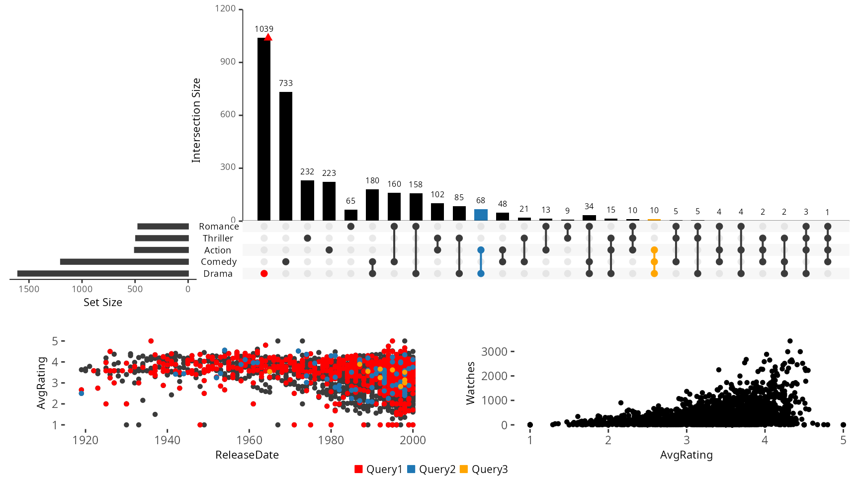

Example 3: Creating a Custom Attribute Plot

Contents of aes_string() along with the scale_color_identity() function are required to pass in aesthetics and to make sure the correct colors are applied. A plot.margin of c(0.5,0,0,1) is recommended.

myplot <- function(mydata,x,y){
    plot <- (ggplot(data = mydata, aes_string(x=x, y=y, colour = "color")) + geom_point() +    scale_color_identity() + theme(plot.margin = unit(c(0,0,0,0), "cm")))
}

another.plot <- function(data, x, y){
  data$decades <- round_any(as.integer(unlist(data[y])), 10, ceiling)
  data <- data[which(data$decades >= 1970), ]
  myplot <- (ggplot(data, aes_string(x=x)) + 
               geom_density(aes(fill=factor(decades)), alpha = 0.4)
             +theme(plot.margin = unit(c(0,0,0,0), "cm"), legend.key.size = unit(0.4,"cm")))
}

Example of applying the myplot custom attribute plot defined above to the data.

upset(movies, main.bar.color = "black", queries = list(list(query = intersects, params = list("Drama"), color = "red", active = F), list(query = intersects, params = list("Action", "Drama"), active = T), list(query = intersects, params = list("Drama", "Comedy", "Action"), color = "orange", active = T)), attribute.plots = list(gridrows = 45, plots = list(list(plot = myplot, x = "ReleaseDate", y = "AvgRating", queries = T), list(plot = another.plot, x = "AvgRating", y = "ReleaseDate", queries = F)), ncols = 2))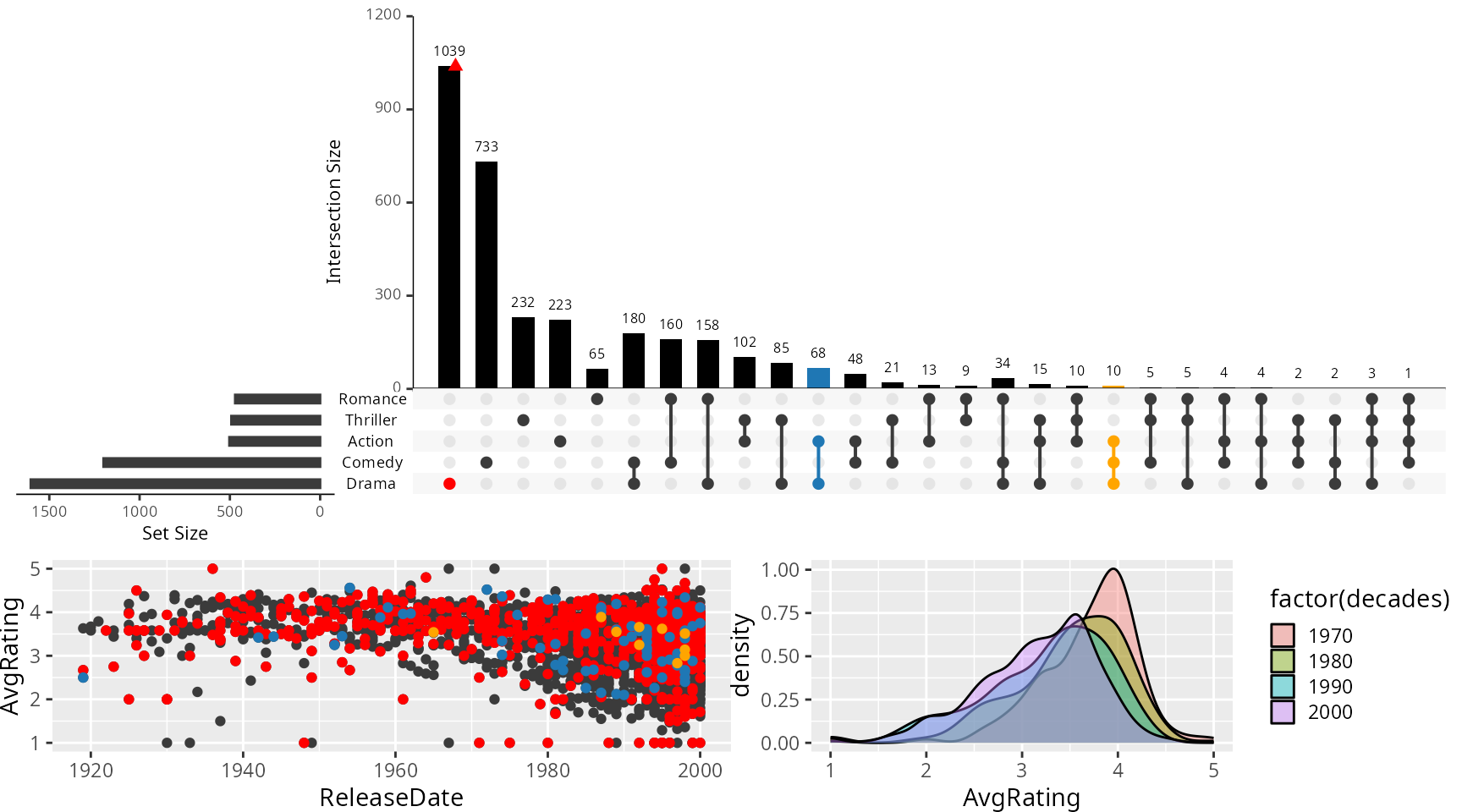

Example 4: Applying Everything at Once

Combining the built-in scatter plot and histogram plot with the myplot custom plot defined in the example above.

upset(movies, main.bar.color = "black", mb.ratio = c(0.5,0.5), queries = list(list(query = intersects, params = list("Drama"), color = "red", active = F), list(query = intersects, params = list("Action", "Drama"), active = T), list(query = intersects, params = list("Drama", "Comedy", "Action"), color = "orange", active = T)), attribute.plots = list(gridrows=50, plots = list(list(plot = histogram, x = "ReleaseDate", queries = F), list(plot = scatter_plot, x = "ReleaseDate", y = "AvgRating", queries = T),list(plot = myplot, x = "AvgRating", y = "Watches", queries = F)), ncols = 3))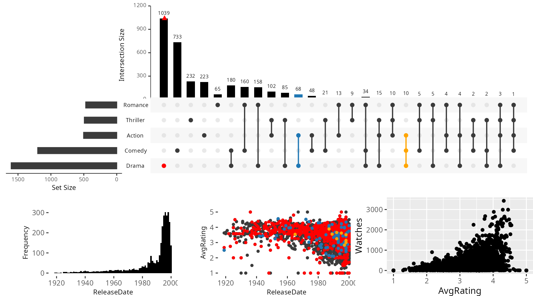

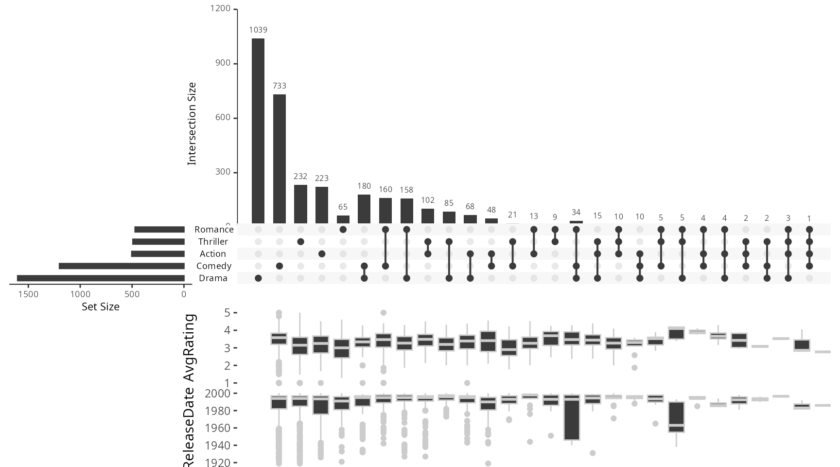
Example 5: Intersection Box Plots

Box plots that show the distribution of an attribute across all intersections. Can display a maximum of two box plot summaries at once. The boxplot.summary parameter takes a vector of one or two attribute names.

upset(movies, boxplot.summary = c("AvgRating", "ReleaseDate"))