Simulate Power of 2-Sample Test for Survival under Complex Conditions

Given functions to generate random variables for survival times and censoring times, spower simulates the power of a user-given 2-sample test for censored data. By default, the logrank (Cox 2-sample) test is used, and a logrank function for comparing 2 groups is provided. Optionally a Cox model is fitted for each each simulated dataset and the log hazard ratios are saved (this requires the survival package). A print method prints various measures from these. For composing R functions to generate random survival times under complex conditions, the Quantile2 function allows the user to specify the intervention:control hazard ratio as a function of time, the probability of a control subject actually receiving the intervention (dropin) as a function of time, and the probability that an intervention subject receives only the control agent as a function of time (non-compliance, dropout). 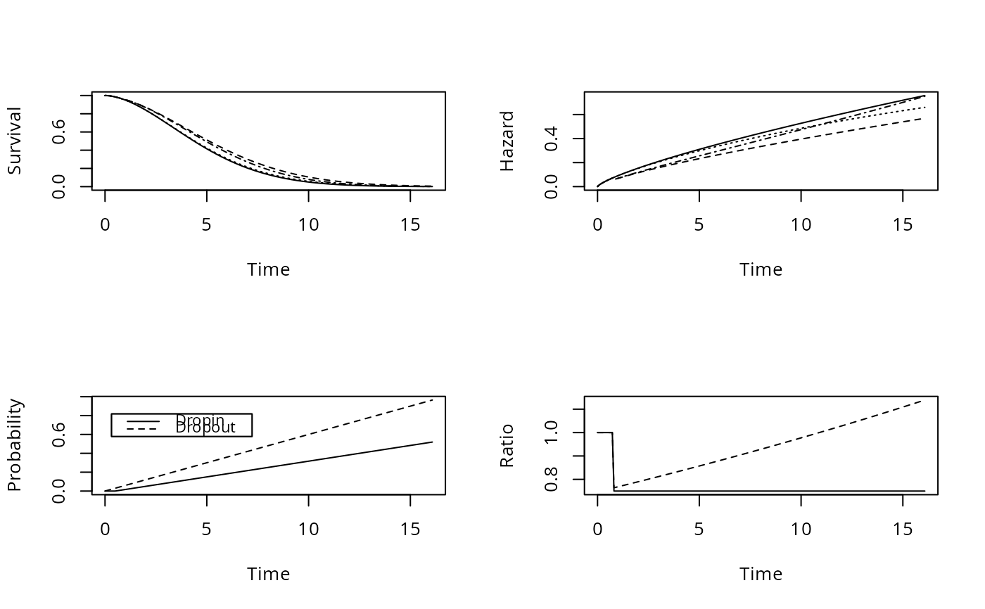Quantile2 returns a function that generates either control or intervention uncensored survival times subject to non-constant treatment effect, dropin, and dropout. There is a plot method for plotting the results of Quantile2, which will aid in understanding the effects of the two types of non-compliance and non-constant treatment effects. Quantile2 assumes that the hazard function for either treatment group is a mixture of the control and intervention hazard functions, with mixing proportions defined by the dropin and dropout probabilities. It computes hazards and survival distributions by numerical differentiation and integration using a grid of (by default) 7500 equally-spaced time points.

The logrank function is intended to be used with spower but it can be used by itself. It returns the 1 degree of freedom chi-square statistic, with the associated Pike hazard ratio estimate as an attribute.

The Weibull2 function accepts as input two vectors, one containing two times and one containing two survival probabilities, and it solves for the scale and shape parameters of the Weibull distribution (\(S(t) = e^{-\alpha {t}^{\gamma}}\)) which will yield those estimates. It creates an R function to evaluate survival probabilities from this Weibull distribution. Weibull2 is useful in creating functions to pass as the first argument to Quantile2.

The Lognorm2 and Gompertz2 functions are similar to Weibull2 except that they produce survival functions for the log-normal and Gompertz distributions.

When cox=TRUE is specified to spower, the analyst may wish to extract the two margins of error by using the print method for spower objects (see example below) and take the maximum of the two.

Usage

spower(rcontrol, rinterv, rcens, nc, ni, 
       test=logrank, cox=FALSE, nsim=500, alpha=0.05, pr=TRUE)

# S3 method for class 'spower'
print(x, conf.int=.95, ...)

Quantile2(scontrol, hratio, 
          dropin=function(times)0, dropout=function(times)0,
          m=7500, tmax, qtmax=.001, mplot=200, pr=TRUE, ...)

# S3 method for class 'Quantile2'
print(x, ...)

# S3 method for class 'Quantile2'
plot(x, 
     what=c("survival", "hazard", "both", "drop", "hratio", "all"),
     dropsep=FALSE, lty=1:4, col=1, xlim, ylim=NULL,
     label.curves=NULL, ...)

logrank(S, group)

Gompertz2(times, surv)
Lognorm2(times, surv)
Weibull2(times, surv)

Arguments

rcontrol: a function of n which returns n random uncensored failure times for the control group. spower assumes that non-compliance (dropin) has been taken into account by this function.
rinterv: similar to rcontrol but for the intervention group
rcens: a function of n which returns n random censoring times. It is assumed that both treatment groups have the same censoring distribution.
nc: number of subjects in the control group
ni: number in the intervention group
scontrol: a function of a time vector which returns the survival probabilities for the control group at those times assuming that all patients are compliant.
hratio: a function of time which specifies the intervention:control hazard ratio (treatment effect)
x: an object of class “Quantile2” created by Quantile2, or of class “spower” created by spower
conf.int: confidence level for determining fold-change margins of error in estimating the hazard ratio
S: a Surv object or other two-column matrix for right-censored survival times
group: group indicators have length equal to the number of rows in S argument.
times: a vector of two times
surv: a vector of two survival probabilities
test: any function of a Surv object and a grouping variable which computes a chi-square for a two-sample censored data test. The default is logrank.
cox: If true TRUE the two margins of error are available by using the print method for spower objects (see example below) and taking the maximum of the two.
nsim: number of simulations to perform (default=500)
alpha: type I error (default=.05)
pr: If FALSE prevents spower from printing progress notes for simulations. If FALSE prevents Quantile2 from printing tmax when it calculates tmax.
dropin: a function of time specifying the probability that a control subject actually is treated with the new intervention at the corresponding time
dropout: a function of time specifying the probability of an intervention subject dropping out to control conditions. As a function of time, dropout specifies the probability that a patient is treated with the control therapy at time t. dropin and dropout form mixing proportions for control and intervention hazard functions.
m: number of time points used for approximating functions (default is 7500)
tmax: maximum time point to use in the grid of m times. Default is the time such that scontrol(time) is qtmax.
qtmax: survival probability corresponding to the last time point used for approximating survival and hazard functions. Default is 0.001. For qtmax of the time for which a simulated time is needed which corresponds to a survival probability of less than qtmax, the simulated value will be tmax.
mplot: number of points used for approximating functions for use in plotting (default is 200 equally spaced points)
...: optional arguments passed to the scontrol function when it's evaluated by Quantile2. Unused for print.spower.
what: a single character constant (may be abbreviated) specifying which functions to plot. The default is "both" meaning both survival and hazard functions. Specify what="drop" to just plot the dropin and dropout functions, what="hratio" to plot the hazard ratio functions, or "all" to make 4 separate plots showing all functions (6 plots if dropsep=TRUE).
dropsep: If TRUE makes plot.Quantile2 separate pure and contaminated functions onto separate plots
lty: vector of line types
col: vector of colors
xlim: optional x-axis limits
ylim: optional y-axis limits
label.curves: optional list which is passed as the opts argument to labcurve.

Value

spower returns the power estimate (fraction of simulated chi-squares greater than the alpha-critical value). If cox=TRUE, spower returns an object of class “spower” containing the power and various other quantities.

Quantile2 returns an R function of class “Quantile2” with attributes that drive the plot method. The major attribute is a list containing several lists. Each of these sub-lists contains a Time vector along with one of the following: survival probabilities for either treatment group and with or without contamination caused by non-compliance, hazard rates in a similar way, intervention:control hazard ratio function with and without contamination, and dropin and dropout functions.

logrank returns a single chi-square statistic and an attribute hr which is the Pike hazard ratio estimate.

Weibull2, Lognorm2 and Gompertz2 return an R function with three arguments, only the first of which (the vector of times) is intended to be specified by the user.

Side Effects

spower prints the interation number every 10 iterations if pr=TRUE.

Author

Frank Harrell
Department of Biostatistics
Vanderbilt University School of Medicine
fh@fharrell.com

References

Lakatos E (1988): Sample sizes based on the log-rank statistic in complex clinical trials. Biometrics 44:229–241 (Correction 44:923).

Cuzick J, Edwards R, Segnan N (1997): Adjusting for non-compliance and contamination in randomized clinical trials. Stat in Med 16:1017–1029.

Cook, T (2003): Methods for mid-course corrections in clinical trials with survival outcomes. Stat in Med 22:3431–3447.

Barthel FMS, Babiker A et al (2006): Evaluation of sample size and power for multi-arm survival trials allowing for non-uniform accrual, non-proportional hazards, loss to follow-up and cross-over. Stat in Med 25:2521–2542.

Examples

# Simulate a simple 2-arm clinical trial with exponential survival so
# we can compare power simulations of logrank-Cox test with cpower()
# Hazard ratio is constant and patients enter the study uniformly
# with follow-up ranging from 1 to 3 years
# Drop-in probability is constant at .1 and drop-out probability is
# constant at .175.  Two-year survival of control patients in absence
# of drop-in is .8 (mortality=.2).  Note that hazard rate is -log(.8)/2
# Total sample size (both groups combined) is 1000
# % mortality reduction by intervention (if no dropin or dropout) is 25
# This corresponds to a hazard ratio of 0.7283 (computed by cpower)


cpower(2, 1000, .2, 25, accrual=2, tmin=1, 
       noncomp.c=10, noncomp.i=17.5)
#> 
#> Accrual duration: 2 y  Minimum follow-up: 1 y
#> 
#> Total sample size: 1000 
#> 
#> Alpha= 0.05 
#> 
#> 2-year Mortalities
#>      Control Intervention 
#>         0.20         0.15 
#> 
#> Hazard Rates
#>      Control Intervention 
#>       0.1116       0.0813 
#> 
#> Probabilities of an Event During Study
#>      Control Intervention 
#>        0.198        0.149 
#> 
#> Expected Number of Events
#>      Control Intervention 
#>         99.2         74.5 
#> 
#> Hazard ratio: 0.728 
#> 
#> Drop-in rate (controls):10%
#> Non-adherence rate (intervention):17.5%
#> Effective hazard ratio with non-compliance: 0.795 
#> Standard deviation of log hazard ratio: 0.153 
#> Power 
#> 0.323 


ranfun <- Quantile2(function(x)exp(log(.8)/2*x),
                    hratio=function(x)0.7283156,
                    dropin=function(x).1,
                    dropout=function(x).175)
#> 
#> Interval of time for evaluating functions:[0, 61.9 ]
#> 


rcontrol <- function(n) ranfun(n, what='control')
rinterv  <- function(n) ranfun(n, what='int')
rcens    <- function(n) runif(n, 1, 3)


set.seed(11)   # So can reproduce results
spower(rcontrol, rinterv, rcens, nc=500, ni=500, 
       test=logrank, nsim=50)  # normally use nsim=500 or 1000
#> 10 
20 
30 
40 
50 

#> [1] 0.24

if (FALSE) { # \dontrun{
# Run the same simulation but fit the Cox model for each one to
# get log hazard ratios for the purpose of assessing the tightness
# confidence intervals that are likely to result

set.seed(11)
u <- spower(rcontrol, rinterv, rcens, nc=500, ni=500, 
       test=logrank, nsim=50, cox=TRUE)
u
v <- print(u)
v[c('MOElower','MOEupper','SE')]
} # }

# Simulate a 2-arm 5-year follow-up study for which the control group's
# survival distribution is Weibull with 1-year survival of .95 and
# 3-year survival of .7.  All subjects are followed at least one year,
# and patients enter the study with linearly increasing probability  after that
# Assume there is no chance of dropin for the first 6 months, then the
# probability increases linearly up to .15 at 5 years
# Assume there is a linearly increasing chance of dropout up to .3 at 5 years
# Assume that the treatment has no effect for the first 9 months, then
# it has a constant effect (hazard ratio of .75)


# First find the right Weibull distribution for compliant control patients
sc <- Weibull2(c(1,3), c(.95,.7))
sc
#> function (times = NULL, alpha = 0.0512932943875506, gamma = 1.76519490623438) 
#> {
#>     exp(-alpha * (times^gamma))
#> }
#> <environment: 0x5e2f8d492968>


# Inverse cumulative distribution for case where all subjects are followed
# at least a years and then between a and b years the density rises
# as (time - a) ^ d is a + (b-a) * u ^ (1/(d+1))


rcens <- function(n) 1 + (5-1) * (runif(n) ^ .5)
# To check this, type hist(rcens(10000), nclass=50)


# Put it all together


f <- Quantile2(sc, 
      hratio=function(x)ifelse(x<=.75, 1, .75),
      dropin=function(x)ifelse(x<=.5, 0, .15*(x-.5)/(5-.5)),
      dropout=function(x).3*x/5)
#> 
#> Interval of time for evaluating functions:[0, 16.1 ]
#> 


par(mfrow=c(2,2))
# par(mfrow=c(1,1)) to make legends fit
plot(f, 'all', label.curves=list(keys='lines'))
#> Warning: no empty rectangle was large enough
#> No empty area large enough for automatic key positioning.  Specify keyloc or cex.
#> Width and height of key as computed by key(), in data units: 11.823  0.412 
#> Warning: no empty rectangle was large enough
#> No empty area large enough for automatic key positioning.  Specify keyloc or cex.
#> Width and height of key as computed by key(), in data units: 11.537  0.312 

#> Warning: no empty rectangle was large enough
#> No empty area large enough for automatic key positioning.  Specify keyloc or cex.
#> Width and height of key as computed by key(), in data units: 16.6035  0.0962 


rcontrol <- function(n) f(n, 'control')
rinterv  <- function(n) f(n, 'intervention')


set.seed(211)
spower(rcontrol, rinterv, rcens, nc=350, ni=350, 
       test=logrank, nsim=50)  # normally nsim=500 or more
#> 10 
20 
30 
40 
50 

#> [1] 0.5
par(mfrow=c(1,1))

# Compose a censoring time generator function such that at 1 year
# 5% of subjects are accrued, at 3 years 70% are accured, and at 10
# years 100% are accrued.  The trial proceeds two years past the last
# accrual for a total of 12 years of follow-up for the first subject.
# Use linear interporation between these 3 points

rcens <- function(n)
{
  times <- c(0,1,3,10)
  accrued <- c(0,.05,.7,1)
  # Compute inverse of accrued function at U(0,1) random variables
  accrual.times <- approx(accrued, times, xout=runif(n))$y
  censor.times <- 12 - accrual.times
  censor.times
}

censor.times <- rcens(500)
# hist(censor.times, nclass=20)
accrual.times <- 12 - censor.times
# Ecdf(accrual.times)
# lines(c(0,1,3,10), c(0,.05,.7,1), col='red')
# spower(..., rcens=rcens, ...)

if (FALSE) { # \dontrun{
# To define a control survival curve from a fitted survival curve
# with coordinates (tt, surv) with tt[1]=0, surv[1]=1:

Scontrol <- function(times, tt, surv) approx(tt, surv, xout=times)$y
tt <- 0:6
surv <- c(1, .9, .8, .75, .7, .65, .64)
formals(Scontrol) <- list(times=NULL, tt=tt, surv=surv)

# To use a mixture of two survival curves, with e.g. mixing proportions
# of .2 and .8, use the following as a guide:
#
# Scontrol <- function(times, t1, s1, t2, s2)
#  .2*approx(t1, s1, xout=times)$y + .8*approx(t2, s2, xout=times)$y
# t1 <- ...; s1 <- ...; t2 <- ...; s2 <- ...;
# formals(Scontrol) <- list(times=NULL, t1=t1, s1=s1, t2=t2, s2=s2)

# Check that spower can detect a situation where generated censoring times
# are later than all failure times

rcens <- function(n) runif(n, 0, 7)
f <- Quantile2(scontrol=Scontrol, hratio=function(x).8, tmax=6)
cont <- function(n) f(n, what='control')
int  <- function(n) f(n, what='intervention')
spower(rcontrol=cont, rinterv=int, rcens=rcens, nc=300, ni=300, nsim=20)

# Do an unstratified logrank test
library(survival)
# From SAS/STAT PROC LIFETEST manual, p. 1801
days <- c(179,256,262,256,255,224,225,287,319,264,237,156,270,257,242,
          157,249,180,226,268,378,355,319,256,171,325,325,217,255,256,
          291,323,253,206,206,237,211,229,234,209)
status <- c(1,1,1,1,1,0,1,1,1,1,0,1,1,1,1,1,1,1,1,0,
            0,rep(1,19))
treatment <- c(rep(1,10), rep(2,10), rep(1,10), rep(2,10))
sex <- Cs(F,F,M,F,M,F,F,M,M,M,F,F,M,M,M,F,M,F,F,M,
          M,M,M,M,F,M,M,F,F,F,M,M,M,F,F,M,F,F,F,F)
data.frame(days, status, treatment, sex)
table(treatment, status)
logrank(Surv(days, status), treatment)  # agrees with p. 1807
# For stratified tests the picture is puzzling.
# survdiff(Surv(days,status) ~ treatment + strata(sex))$chisq
# is 7.246562, which does not agree with SAS (7.1609)
# But summary(coxph(Surv(days,status) ~ treatment + strata(sex)))
# yields 7.16 whereas summary(coxph(Surv(days,status) ~ treatment))
# yields 5.21 as the score test, not agreeing with SAS or logrank() (5.6485)
} # }