Power of Cox/log-rank Two-Sample Test
cpower.RdAssumes exponential distributions for both treatment groups. Uses the George-Desu method along with formulas of Schoenfeld that allow estimation of the expected number of events in the two groups. To allow for drop-ins (noncompliance to control therapy, crossover to intervention) and noncompliance of the intervention, the method of Lachin and Foulkes is used.
Arguments
- tref
time at which mortalities estimated
- n
total sample size (both groups combined). If allocation is unequal so that there are not
n/2observations in each group, you may specify the sample sizes inncandni.- mc
tref-year mortality, control
- r
% reduction in
mcby intervention- accrual
duration of accrual period
- tmin
minimum follow-up time
- noncomp.c
% non-compliant in control group (drop-ins)
- noncomp.i
% non-compliant in intervention group (non-adherers)
- alpha
type I error probability. A 2-tailed test is assumed.
- nc
number of subjects in control group
- ni
number of subjects in intervention group.
ncandniare specified exclusive ofn.- pr
set to
FALSEto suppress printing of details
Details
For handling noncompliance, uses a modification of formula (5.4) of
Lachin and Foulkes. Their method is based on a test for the difference
in two hazard rates, whereas cpower is based on testing the difference
in two log hazards. It is assumed here that the same correction factor
can be approximately applied to the log hazard ratio as Lachin and Foulkes applied to
the hazard difference.
Note that Schoenfeld approximates the variance
of the log hazard ratio by 4/m, where m is the total number of events,
whereas the George-Desu method uses the slightly better 1/m1 + 1/m2.
Power from this function will thus differ slightly from that obtained with
the SAS samsizc program.
Author
Frank Harrell
Department of Biostatistics
Vanderbilt University
fh@fharrell.com
References
Peterson B, George SL: Controlled Clinical Trials 14:511–522; 1993.
Lachin JM, Foulkes MA: Biometrics 42:507–519; 1986.
Schoenfeld D: Biometrics 39:499–503; 1983.
Examples
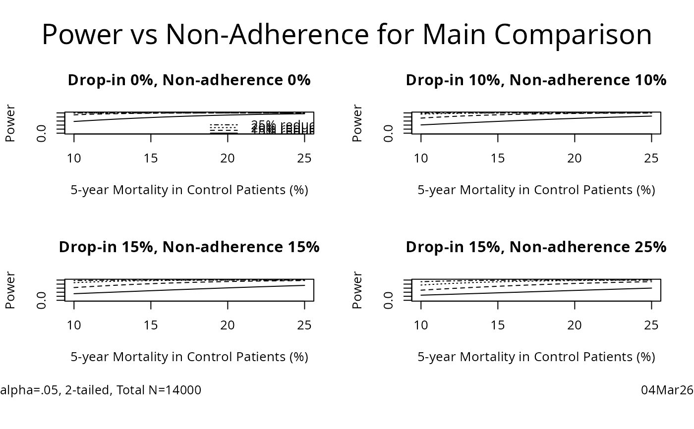
#In this example, 4 plots are drawn on one page, one plot for each
#combination of noncompliance percentage. Within a plot, the
#5-year mortality % in the control group is on the x-axis, and
#separate curves are drawn for several % reductions in mortality
#with the intervention. The accrual period is 1.5y, with all
#patients followed at least 5y and some 6.5y.
par(mfrow=c(2,2),oma=c(3,0,3,0))
morts <- seq(10,25,length=50)
red <- c(10,15,20,25)
for(noncomp in c(0,10,15,-1)) {
if(noncomp>=0) nc.i <- nc.c <- noncomp else {nc.i <- 25; nc.c <- 15}
z <- paste("Drop-in ",nc.c,"%, Non-adherence ",nc.i,"%",sep="")
plot(0,0,xlim=range(morts),ylim=c(0,1),
xlab="5-year Mortality in Control Patients (%)",
ylab="Power",type="n")
title(z)
cat(z,"\n")
lty <- 0
for(r in red) {
lty <- lty+1
power <- morts
i <- 0
for(m in morts) {
i <- i+1
power[i] <- cpower(5, 14000, m/100, r, 1.5, 5, nc.c, nc.i, pr=FALSE)
}
lines(morts, power, lty=lty)
}
if(noncomp==0)legend(18,.55,rev(paste(red,"% reduction",sep="")),
lty=4:1,bty="n")
}
#> Drop-in 0%, Non-adherence 0%
#> Drop-in 10%, Non-adherence 10%
#> Drop-in 15%, Non-adherence 15%
#> Drop-in 15%, Non-adherence 25%
mtitle("Power vs Non-Adherence for Main Comparison",
ll="alpha=.05, 2-tailed, Total N=14000",cex.l=.8)
 #
# Point sample size requirement vs. mortality reduction
# Root finder (uniroot()) assumes needed sample size is between
# 1000 and 40000
#
nc.i <- 25; nc.c <- 15; mort <- .18
red <- seq(10,25,by=.25)
samsiz <- red
i <- 0
for(r in red) {
i <- i+1
samsiz[i] <- uniroot(function(x) cpower(5, x, mort, r, 1.5, 5,
nc.c, nc.i, pr=FALSE) - .8,
c(1000,40000))$root
}
samsiz <- samsiz/1000
par(mfrow=c(1,1))
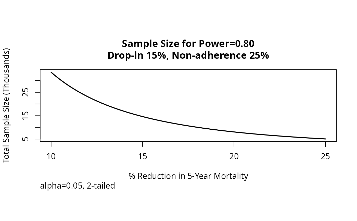
plot(red, samsiz, xlab='% Reduction in 5-Year Mortality',
ylab='Total Sample Size (Thousands)', type='n')
lines(red, samsiz, lwd=2)
title('Sample Size for Power=0.80\nDrop-in 15%, Non-adherence 25%')
title(sub='alpha=0.05, 2-tailed', adj=0)
#
# Point sample size requirement vs. mortality reduction
# Root finder (uniroot()) assumes needed sample size is between
# 1000 and 40000
#
nc.i <- 25; nc.c <- 15; mort <- .18
red <- seq(10,25,by=.25)
samsiz <- red
i <- 0
for(r in red) {
i <- i+1
samsiz[i] <- uniroot(function(x) cpower(5, x, mort, r, 1.5, 5,
nc.c, nc.i, pr=FALSE) - .8,
c(1000,40000))$root
}
samsiz <- samsiz/1000
par(mfrow=c(1,1))
plot(red, samsiz, xlab='% Reduction in 5-Year Mortality',
ylab='Total Sample Size (Thousands)', type='n')
lines(red, samsiz, lwd=2)
title('Sample Size for Power=0.80\nDrop-in 15%, Non-adherence 25%')
title(sub='alpha=0.05, 2-tailed', adj=0)