Label Curves, Make Keys, and Interactively Draw Points and Curves
labcurve.Rdlabcurve optionally draws a set of curves then labels the curves.
A variety of methods for drawing labels are implemented, ranging from
positioning using the mouse to automatic labeling to automatic placement
of key symbols with manual placement of key legends to automatic
placement of legends. For automatic positioning of labels or keys, a
curve is labeled at a point that is maximally separated from all of the
other curves. Gaps occurring when curves do not start or end at the
same x-coordinates are given preference for positioning labels. If
labels are offset from the curves (the default behaviour), if the
closest curve to curve i is above curve i, curve i is labeled below its
line. If the closest curve is below curve i, curve i is labeled above
its line. These directions are reversed if the resulting labels would
appear outside the plot region.
Both ordinary lines and step functions are handled, and there is an option to draw the labels at the same angle as the curve within a local window.
Unless the mouse is used to position labels or plotting symbols are
placed along the curves to distinguish them, curves are examined at 100
(by default) equally spaced points over the range of x-coordinates in
the current plot area. Linear interpolation is used to get
y-coordinates to line up (step function or constant interpolation is
used for step functions). There is an option to instead examine all
curves at the set of unique x-coordinates found by unioning the
x-coordinates of all the curves. This option is especially useful when
plotting step functions. By setting adj="auto" you can have
labcurve try to optimally left- or right-justify labels depending
on the slope of the curves at the points at which labels would be
centered (plus a vertical offset). This is especially useful when
labels must be placed on steep curve sections.
You can use the on top method to write (short) curve names
directly on the curves (centered on the y-coordinate). This is
especially useful when there are many curves whose full labels would run
into each other. You can plot letters or numbers on the curves, for
example (using the keys option), and have labcurve use the
key function to provide long labels for these short ones (see the
end of the example). There is another option for connecting labels to
curves using arrows. When keys is a vector of integers, it is
taken to represent plotting symbols (pchs), and these symbols are
plotted at equally-spaced x-coordinates on each curve (by default, using
5 points per curve). The points are offset in the x-direction between
curves so as to minimize the chance of collisions.
To add a legend defining line types, colors, or line widths with no
symbols, specify keys="lines", e.g., labcurve(curves,
keys="lines", lty=1:2).
putKey provides a different way to use key() by allowing
the user to specify vectors for labels, line types, plotting characters,
etc. Elements that do not apply (e.g., pch for lines
(type="l")) may be NA. When a series of points is
represented by both a symbol and a line, the corresponding elements of
both pch and lty, col., or lwd will be
non-missing.
putKeyEmpty, given vectors of all the x-y coordinates that have been
plotted, uses largest.empty to find the largest empty rectangle large
enough to hold the key, and draws the key using putKey.
drawPlot is a simple mouse-driven function for drawing series of
lines, step functions, polynomials, Bezier curves, and points, and
automatically labeling the point groups using labcurve or
putKeyEmpty. When drawPlot is invoked it creates
temporary functions Points, Curve, and Abline.
The user calls these functions inside
the call to drawPlot to define groups of points in the order they
are defined with the mouse. Abline is used to call abline
and not actually great a group of points. For some curve types, the
curve generated to represent the corresponding series of points is drawn
after all points are entered for that series, and this curve may be
different than the simple curve obtained by connecting points at the
mouse clicks. For example, to draw a general smooth Bezier curve the
user need only click on a few points, and she must overshoot the final
curve coordinates to define the curve. The originally entered points
are not erased once the curve is drawn. The same goes for step
functions and polynomials. If you plot() the object returned by
drawPlot, however, only final curves will be shown. The last
examples show how to use drawPlot.
The largest.empty function finds the largest rectangle that is large
enough to hold a rectangle of a given height and width, such that the
rectangle does not contain any of a given set of points. This is
used by labcurve and putKeyEmpty to position keys at the most
empty part of an existing plot. The default method was created by Hans
Borchers.
Usage
labcurve(curves, labels=names(curves),
         method=NULL, keys=NULL, keyloc=c("auto","none"),
         type="l", step.type=c("left", "right"),
         xmethod=if(any(type=="s")) "unique" else "grid",
         offset=NULL, xlim=NULL,
         tilt=FALSE, window=NULL, npts=100, cex=NULL,
         adj="auto", angle.adj.auto=30,
         lty=pr$lty, lwd=pr$lwd, col.=pr$col, transparent=TRUE,
         arrow.factor=1, point.inc=NULL, opts=NULL, key.opts=NULL,
         empty.method=c('area','maxdim'), numbins=25,
         pl=!missing(add), add=FALSE,
         ylim=NULL, xlab="", ylab="",
         whichLabel=1:length(curves),
         grid=FALSE, xrestrict=NULL, ...)

putKey(z, labels, type, pch, lty, lwd,
       cex=par('cex'), col=rep(par('col'),nc),
       transparent=TRUE, plot=TRUE, key.opts=NULL, grid=FALSE)

putKeyEmpty(x, y, labels, type=NULL,
            pch=NULL, lty=NULL, lwd=NULL,
            cex=par('cex'), col=rep(par('col'),nc),
            transparent=TRUE, plot=TRUE, key.opts=NULL,
            empty.method=c('area','maxdim'),
            numbins=25,
            xlim=pr$usr[1:2], ylim=pr$usr[3:4], grid=FALSE)

drawPlot(..., xlim=c(0,1), ylim=c(0,1), xlab='', ylab='',
         ticks=c('none','x','y','xy'),
         key=FALSE, opts=NULL)

# Points(label=' ', type=c('p','r'),
#        n, pch=pch.to.use[1], cex=par('cex'), col=par('col'),
#        rug = c('none','x','y','xy'), ymean)

# Curve(label=' ',
#       type=c('bezier','polygon','linear','pol','loess','step','gauss'),
#       n=NULL, lty=1, lwd=par('lwd'), col=par('col'), degree=2,
#      evaluation=100, ask=FALSE)

# Abline(\dots)

# S3 method for class 'drawPlot'
plot(x, xlab, ylab, ticks,
     key=x$key, keyloc=x$keyloc, ...)

largest.empty(x, y, width=0, height=0,
              numbins=25, method=c('exhaustive','rexhaustive','area','maxdim'),
              xlim=pr$usr[1:2], ylim=pr$usr[3:4],
              pl=FALSE, grid=FALSE)
Arguments
- curves
a list of lists, each of which have at least two components: a vector of
xvalues and a vector of correspondingyvalues.curvesis mandatory except whenmethod="mouse"or"locator", in which caselabelsis mandatory. Each list incurvesmay optionally have any of the parameterstype,lty,lwd, orcolfor that curve, as defined below (see one of the last examples).- z
a two-element list specifying the coordinate of the center of the key, e.g.
locator(1)to use the mouse for positioning- labels
For
labcurve, a vector of character strings used to label curves (which may contain newline characters to stack labels vertically). The default labels are taken from the names of thecurveslist. Settinglabels=FALSEwill suppress drawing any labels (forlabcurveonly). ForputKeyandputKeyEmptyis a vector of character strings specifying group labels- x
see below
- y
for
putKeyEmptyandlargest.empty,xandyare same-length vectors specifying points that have been plotted.xcan also be an object created bydrawPlot.- ...
For
drawPlotis a series of invocations ofPointsandCurve(see example). Any number of point groups can be defined in this way. ForAblinethese may be any arguments toabline. Forlabcurve, other parameters to pass totext.- width
see below
- height
for
largest.empty, specifies the minimum allowable width inxunits and the minimum allowable height inyunits- method
"offset"(the default) offsets labels at largest gaps between curves, and draws labels beside curves."on top"draws labels on top of the curves (especially good when using keys)."arrow"draws arrows connecting labels to the curves."mouse"or"locator"positions labels according to mouse clicks. Ifkeysis specified and is an integer vector or is"lines",methoddefaults to"on top". Ifkeysis character,methoddefaults to"offset". Setmethod="none"to suppress all curve labeling and key drawing, which is useful whenpl=TRUEand you only needlabcurveto draw the curves and the rest of the basic graph.For
largest.emptyspecifies the method a rectangle that does not collide with any of the (x,y) points. The default method,'exhaustive', uses a Fortran translation of an R function and algorithm developed by Hans Borchers. The same result, more slowly, may be obtained by using pure R code by specifyingmethod='rexhaustive'. The original algorithms using binning (and the only methods supported for S-Plus) are still available. For all methods, screening of candidate rectangles having at least a given width inx-units ofwidthor having at least a given height iny-units ofheightis possible. Usemethod="area"to use the binning method to find the rectangle having the largest area, ormethod="maxdim"to use the binning method to return with last rectangle searched that had both the largest width and largest height over all previous rectangles.- keys
This causes keys (symbols or short text) to be drawn on or beside curves, and if
keylocis not equal to"none", a legend to be automatically drawn. The legend links keys with full curve labels and optionally with colors and line types. Setkeysto a vector of character strings, or a vector of integers specifying plotting character (pchvalues - seepoints). For the latter case, the default behavior is to plot the symbols periodically, at equally spaced x-coordinates.- keyloc
When
keysis specified,keylocspecifies how the legend is to be positioned for drawing using thekeyfunction intrellis. The default is"auto", for which thelargest.emptyfunction to used to find the most empty part of the plot. If no empty rectangle large enough to hold the key is found, no key will be drawn. Specifykeyloc="none"to suppress drawing a legend, or setkeylocto a 2-element list containing the x and y coordinates for the center of the legend. For example, usekeyloc=locator(1)to click the mouse at the center.keylocspecifies the coordinates of the center of the key to be drawn withplot.drawPlotwhenkey=TRUE.- type
for
labcurve, a scalar or vector of character strings specifying the method that the points in the curves were connected."l"means ordinary connections between points and"s"means step functions. ForputKeyandputKeyEmptyis a vector of plotting types,"l"for regular line,"p"for point,"b"for both point and line, and"n"for none. ForPointsis either"p"(the default) for regular points, or"r"for rugplot (one-dimensional scatter diagram to be drawn using thescat1dfunction). ForCurve,typeis"bezier"(the default) for drawing a smooth Bezier curves (which can represent a non-1-to-1 function such as a circle),"polygon"for orginary line segments,"linear"for a straight line defined by two endpoints,"pol"for adegree-degree polynomial to be fitted to the mouse-clicked points,"step"for a left-step-function,"gauss"to plot a Gaussian density fitted to 3 clicked points,"loess"to use thelowessfunction to smooth the clicked points, or a function to draw a user-specified function, evaluated atevaluationpoints spanning the whole x-axis. For the density the user must click in the left tail, at the highest value (at the mean), and in the right tail, with the two tail values being approximately equidistant from the mean. The density is scaled to fit in the highest value regardless of its area.- step.type
type of step functions used (default is
"left")- xmethod
method for generating the unique set of x-coordinates to examine (see above). Default is
"grid"fortype="l"or"unique"fortype="s".- offset
distance in y-units between the center of the label and the line being labeled. Default is 0.75 times the height of an "m" that would be drawn in a label. For R grid/lattice you must specify offset using the
gridunitfunction, e.g.,offset=unit(2,"native")oroffset=unit(.25,"cm")("native"means data units)- xlim
limits for searching for label positions, and is also used to set up plots when
pl=TRUEandadd=FALSE. Default is total x-axis range for current plot (par("usr")[1:2]). Forlargest.empty,xlimlimits the search for largest rectanges, but it has the same default as above. Forpl=TRUE,add=FALSEyou may want to extendxlimsomewhat to allow large keys to fit, when usingkeyloc="auto". FordrawPlotdefault isc(0,1). When usinglargest.emptywithggplot2,xlimandylimare mandatory.- tilt
set to
TRUEto tilt labels to follow the curves, formethod="offset"whenkeysis not given.- window
width of a window, in x-units, to use in determining the local slope for tilting labels. Default is 0.5 times number of characters in the label times the x-width of an "m" in the current character size and font.
- npts
number of points to use if
xmethod="grid"- cex
character size to pass to
textandkey. Default is currentpar("cex"). ForputKey,putKeyEmpty, andPointsis the size of the plotting symbol.- adj
Default is
"auto"which haslabcurvefigure justification automatically whenmethod="offset". This will cause centering to be used when the local angle of the curve is less thanangle.adj.autoin absolute value, left justification if the angle is larger and either the label is under a curve of positive slope or over a curve of negative slope, and right justification otherwise. For step functions, left justification is used when the label is above the curve and right justifcation otherwise. Setadj=.5to center labels at computed coordinates. Set to 0 for left-justification, 1 for right. Setadjto a vector to vary adjustments over the curves.- angle.adj.auto
see
adj. Does not apply to step functions.- lty
vector of line types which were used to draw the curves. This is only used when keys are drawn. If all of the line types, line widths, and line colors are the same, lines are not drawn in the key.
- lwd
vector of line widths which were used to draw the curves. This is only used when keys are drawn. See
ltyalso.- col.
vector of integer color numbers
- col
vector of integer color numbers for use in curve labels, symbols, lines, and legends. Default is
par("col")for all curves. Seeltyalso.- transparent
Default is
TRUEto makekeydraw transparent legends, i.e., to suppress drawing a solid rectangle background for the legend. Set toFALSEotherwise.- arrow.factor
factor by which to multiply default arrow lengths
- point.inc
When
keysis a vector of integers,point.incspecifies the x-increment between the point symbols that are overlaid periodically on the curves. By default,point.incis equal to the range for the x-axis divided by 5.- opts
an optional list which can be used to specify any of the options to
labcurve, with the usual element name abbreviations allowed. This is useful whenlabcurveis being called from another function. Example:opts=list(method="arrow", cex=.8, np=200). FordrawPlota list oflabcurveoptions to pass aslabcurve(..., opts=).- key.opts
a list of extra arguments you wish to pass to
key(), e.g.,key.opts=list(background=1, between=3). The argument names must be spelled out in full.- empty.method
see below
- numbins
These two arguments are passed to the
largest.emptyfunction'smethodandnumbinsarguments (see below). Forlargest.emptyspecifies the number of bins in which to discretize both thexandydirections for searching for rectangles. Default is 25.- pl
set to
TRUE(or specifyadd) to cause the curves incurvesto be drawn, under the control oftype,lty,lwd,colparameters defined either in thecurveslists or in the separate arguments given tolabcurveor throughopts. Forlargest.empty, setpl=TRUEto show the rectangle the function found by drawing it with a solid color. May not be used underggplot2.- add
By default, when curves are actually drawn by
labcurvea new plot is started. To add to an existing plot, setadd=TRUE.- ylim
When a plot has already been started,
ylimdefaults topar("usr")[3:4]. Whenpl=TRUE,ylimandxlimare determined from the ranges of the data. Specifyylimyourself to take control of the plot construction. In some cases it is advisable to makeylimlarger than usual to allow for automatically-positioned keys. Forlargest.empty,ylimspecifies the limits on the y-axis to limit the search for rectangle. Hereylimdefaults to the same as above, i.e., the range of the y-axis of an open plot frompar. FordrawPlotthe default isc(0,1).- xlab
see below
- ylab
x-axis and y-axis labels when
pl=TRUEandadd=FALSEor fordrawPlot. Defaults to""unless the first curve has names for its first two elements, in which case the names of these elements are taken asxlabandylab.- whichLabel
integer vector corresponding to
curvesspecifying which curves are to be labelled or have a legend- grid
set to
TRUEif the Rgridpackage was used to draw the current plot. This preventslabcurvefrom usingpar("usr")etc. If using Rgridyou can pass coordinates and lengths having arbitrary units, as documented in theunitfunction. This is especially useful foroffset.- xrestrict
When having
labcurvelabel curves where they are most separated, you can restrict the search for this separation point to a range of the x-axis, specified as a 2-vectorxrestrict. This is useful when one part of the curve is very steep. Even though steep regions may have maximum separation, the labels will collide when curves are steep.- pch
vector of plotting characters for
putKeyandputKeyEmpty. Can be any value includingNAwhen only a line is used to indentify the group. Is a single plotting character forPoints, with the default being the next unused value from among 1, 2, 3, 4, 16, 17, 5, 6, 15, 18, 19.- plot
set to
FALSEto keepputKeyorputKeyEmptyfrom actually drawing the key. Instead, the size of the key will be return byputKey, or the coordinates of the key byputKeyEmpty.- ticks
tells
drawPlotwhich axes to draw tick marks and tick labels. Default is"none".- key
for
drawPlotandplot.drawPlot. Default isFALSEso thatlabcurveis used to label points or curves. Set toTRUEto useputKeyEmpty.
Value
labcurve returns an invisible list with components x, y, offset, adj, cex, col, and if tilt=TRUE,
angle. offset is the amount to add to y to draw a label.
offset is negative if the label is drawn below the line.
adj is a vector containing the values 0, .5, 1.
largest.empty returns a list with elements x and y
specifying the coordinates of the center of the rectangle which was
found, and element rect containing the 4 x and y
coordinates of the corners of the found empty rectangle. The
area of the rectangle is also returned.
Details
The internal functions Points, Curve, Abline have
unique arguments as follows.
label:for
PointsandCurveis a single character string to label that group of pointsn:number of points to accept from the mouse. Default is to input points until a right mouse click.
rug:for
Points. Default is"none"to not show the marginal x or y distributions as rug plots, for the points entered. Other possibilities are used to executescat1dto show the marginal distribution of x, y, or both as rug plots.ymean:for
Points, subtracts a constant from each y-coordinate entered to make the overall meanymeandegree:degree of polynomial to fit to points by
Curveevaluation:number of points at which to evaluate Bezier curves, polynomials, and other functions in
Curveask:set
ask=TRUEto give the user the opportunity to try again at specifying points for Bezier curves, step functions, and polynomials
The labcurve function used some code from the function plot.multicurve written
by Rod Tjoelker of The Boeing Company (tjoelker@espresso.rt.cs.boeing.com).
If there is only one curve, a label is placed at the middle x-value,
and no fancy features such as angle or positive/negative offsets are
used.
key is called once (with the argument plot=FALSE) to find the key
dimensions. Then an empty rectangle with at least these dimensions is
searched for using largest.empty. Then key is called again to draw
the key there, using the argument corner=c(.5,.5) so that the center
of the rectangle can be specified to key.
If you want to plot the data, an easier way to use labcurve is
through xYplot as shown in some of its examples.
Author
Frank Harrell
Department of Biostatistics
Vanderbilt University
fh@fharrell.com
Examples
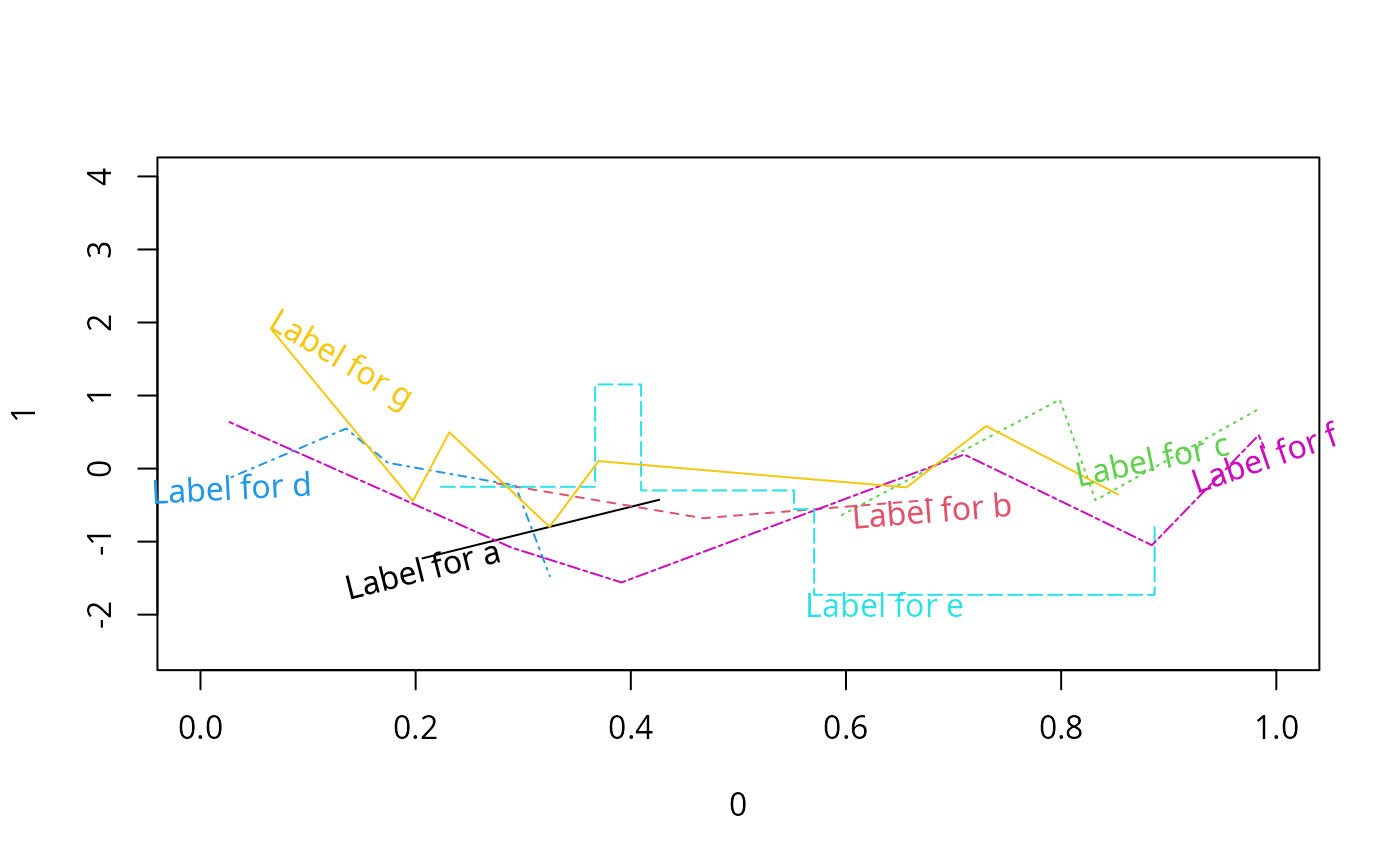
n <- 2:8
m <- length(n)
type <- c('l','l','l','l','s','l','l')
# s=step function l=ordinary line (polygon)
curves <- vector('list', m)
plot(0,1,xlim=c(0,1),ylim=c(-2.5,4),type='n')
set.seed(39)
for(i in 1:m) {
x <- sort(runif(n[i]))
y <- rnorm(n[i])
lines(x, y, lty=i, type=type[i], col=i)
curves[[i]] <- list(x=x,y=y)
}
labels <- paste('Label for',letters[1:m])
labcurve(curves, labels, tilt=TRUE, type=type, col=1:m)
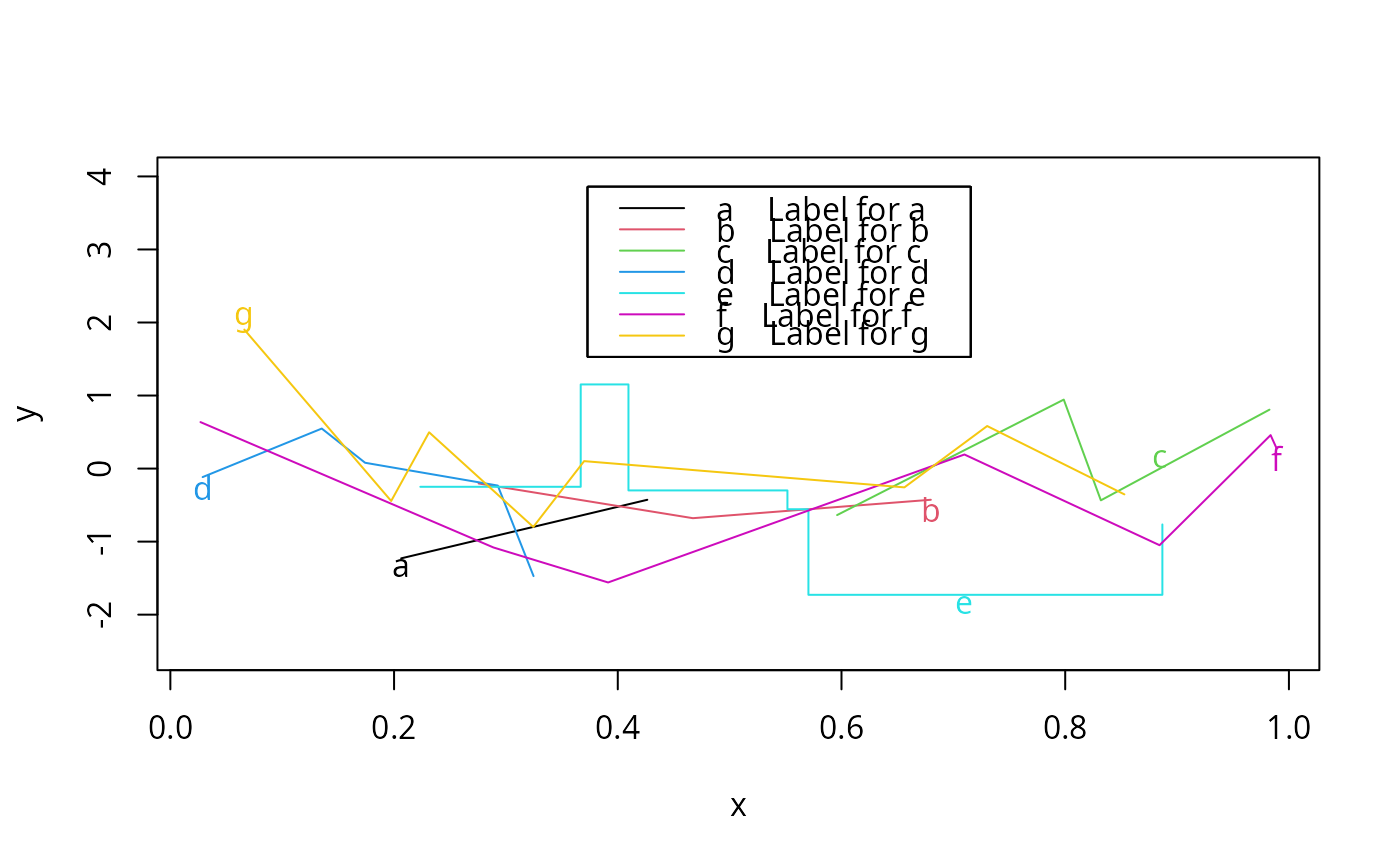
 # Put only single letters on curves at points of
# maximum space, and use key() to define the letters,
# with automatic positioning of the key in the most empty
# part of the plot
# Have labcurve do the plotting, leaving extra space for key
names(curves) <- labels
labcurve(curves, keys=letters[1:m], type=type, col=1:m,
pl=TRUE, ylim=c(-2.5,4))
# Put only single letters on curves at points of
# maximum space, and use key() to define the letters,
# with automatic positioning of the key in the most empty
# part of the plot
# Have labcurve do the plotting, leaving extra space for key
names(curves) <- labels
labcurve(curves, keys=letters[1:m], type=type, col=1:m,
pl=TRUE, ylim=c(-2.5,4))
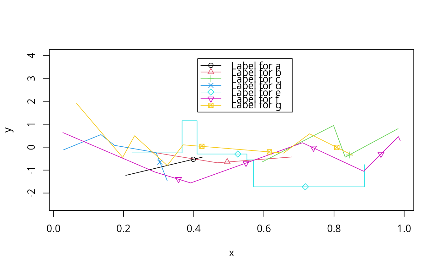
 # Put plotting symbols at equally-spaced points,
# with a key for the symbols, ignoring line types
labcurve(curves, keys=1:m, lty=1, type=type, col=1:m,
pl=TRUE, ylim=c(-2.5,4))
# Put plotting symbols at equally-spaced points,
# with a key for the symbols, ignoring line types
labcurve(curves, keys=1:m, lty=1, type=type, col=1:m,
pl=TRUE, ylim=c(-2.5,4))
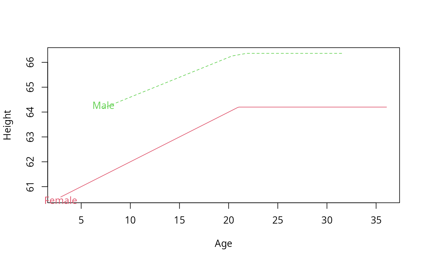
 # Plot and label two curves, with line parameters specified with data
set.seed(191)
ages.f <- sort(rnorm(50,20,7))
ages.m <- sort(rnorm(40,19,7))
height.f <- pmin(ages.f,21)*.2+60
height.m <- pmin(ages.m,21)*.16+63
labcurve(list(Female=list(ages.f,height.f,col=2),
Male =list(ages.m,height.m,col=3,lty='dashed')),
xlab='Age', ylab='Height', pl=TRUE)
# Plot and label two curves, with line parameters specified with data
set.seed(191)
ages.f <- sort(rnorm(50,20,7))
ages.m <- sort(rnorm(40,19,7))
height.f <- pmin(ages.f,21)*.2+60
height.m <- pmin(ages.m,21)*.16+63
labcurve(list(Female=list(ages.f,height.f,col=2),
Male =list(ages.m,height.m,col=3,lty='dashed')),
xlab='Age', ylab='Height', pl=TRUE)
 # add ,keys=c('f','m') to label curves with single letters
# For S-Plus use lty=2
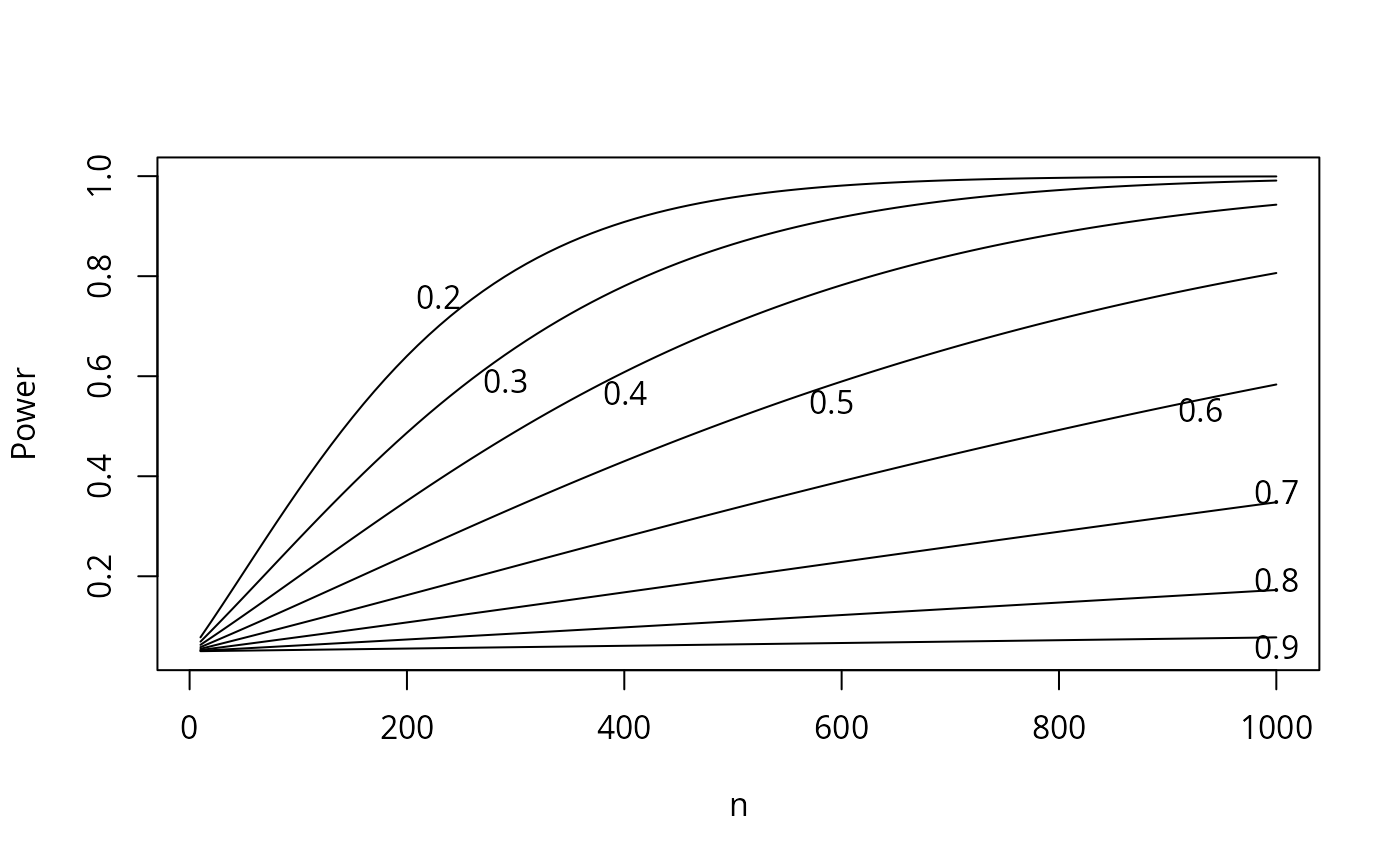
# Plot power for testing two proportions vs. n for various odds ratios,
# using 0.1 as the probability of the event in the control group.
# A separate curve is plotted for each odds ratio, and the curves are
# labeled at points of maximum separation
n <- seq(10, 1000, by=10)
OR <- seq(.2,.9,by=.1)
pow <- lapply(OR, function(or,n)list(x=n,y=bpower(p1=.1,odds.ratio=or,n=n)),
n=n)
names(pow) <- format(OR)
labcurve(pow, pl=TRUE, xlab='n', ylab='Power')
# add ,keys=c('f','m') to label curves with single letters
# For S-Plus use lty=2
# Plot power for testing two proportions vs. n for various odds ratios,
# using 0.1 as the probability of the event in the control group.
# A separate curve is plotted for each odds ratio, and the curves are
# labeled at points of maximum separation
n <- seq(10, 1000, by=10)
OR <- seq(.2,.9,by=.1)
pow <- lapply(OR, function(or,n)list(x=n,y=bpower(p1=.1,odds.ratio=or,n=n)),
n=n)
names(pow) <- format(OR)
labcurve(pow, pl=TRUE, xlab='n', ylab='Power')
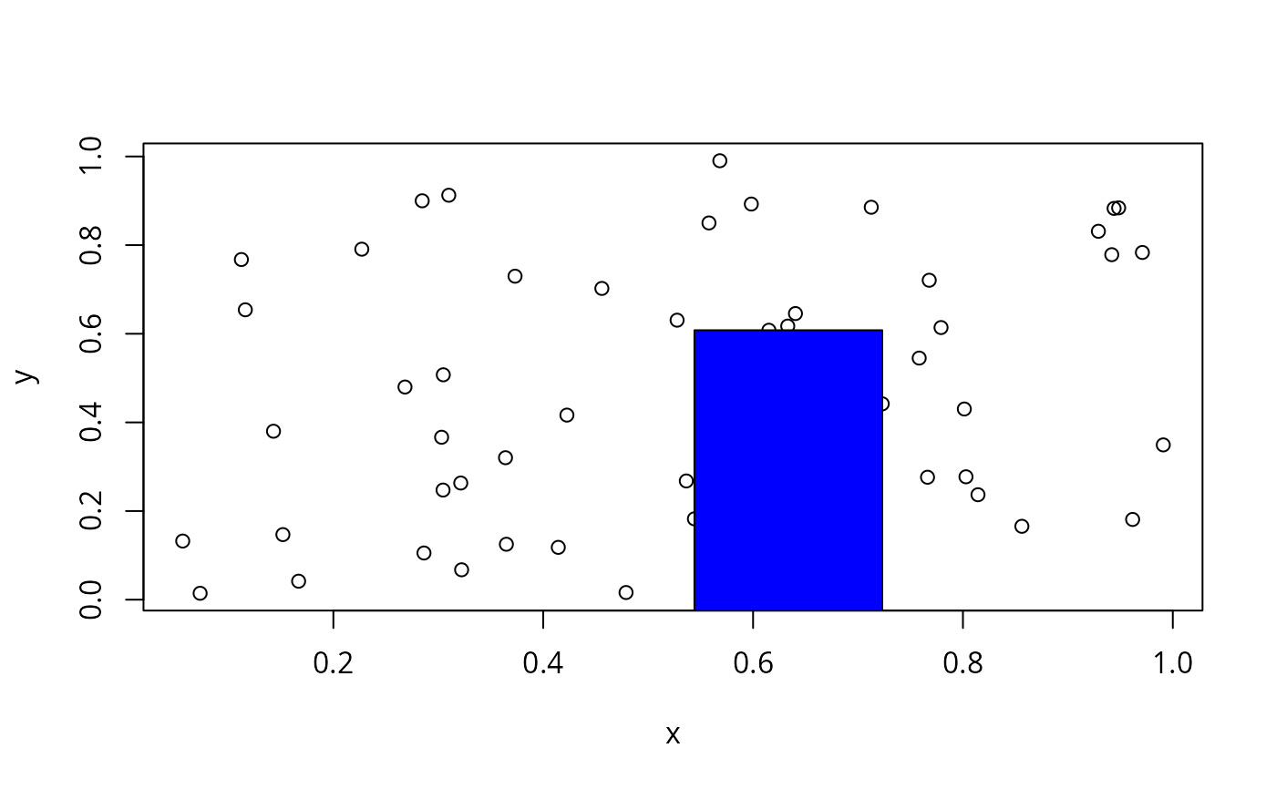
 # Plot some random data and find the largest empty rectangle
# that is at least .1 wide and .1 tall
x <- runif(50)
y <- runif(50)
plot(x, y)
z <- largest.empty(x, y, .1, .1)
z
#> $x
#> [1] 0.634
#>
#> $y
#> [1] 0.292
#>
#> $rect
#> $rect$x
#> [1] 0.544 0.723 0.723 0.544
#>
#> $rect$y
#> [1] -0.0246 -0.0246 0.6080 0.6080
#>
#>
#> $area
#> [1] 0.113
#>
points(z,pch=3) # mark center of rectangle, or
polygon(z$rect, col='blue') # to draw the rectangle, or
# Plot some random data and find the largest empty rectangle
# that is at least .1 wide and .1 tall
x <- runif(50)
y <- runif(50)
plot(x, y)
z <- largest.empty(x, y, .1, .1)
z
#> $x
#> [1] 0.634
#>
#> $y
#> [1] 0.292
#>
#> $rect
#> $rect$x
#> [1] 0.544 0.723 0.723 0.544
#>
#> $rect$y
#> [1] -0.0246 -0.0246 0.6080 0.6080
#>
#>
#> $area
#> [1] 0.113
#>
points(z,pch=3) # mark center of rectangle, or
polygon(z$rect, col='blue') # to draw the rectangle, or
 #key(z$x, z$y, \dots stuff for legend)
# Use the mouse to draw a series of points using one symbol, and
# two smooth curves or straight lines (if two points are clicked),
# none of these being labeled
# d <- drawPlot(Points(), Curve(), Curve())
# plot(d)
if (FALSE) { # \dontrun{
# Use the mouse to draw a Gaussian density, two series of points
# using 2 symbols, one Bezier curve, a step function, and raw data
# along the x-axis as a 1-d scatter plot (rug plot). Draw a key.
# The density function is fit to 3 mouse clicks
# Abline draws a dotted horizontal reference line
d <- drawPlot(Curve('Normal',type='gauss'),
Points('female'), Points('male'),
Curve('smooth',ask=TRUE,lty=2), Curve('step',type='s',lty=3),
Points(type='r'), Abline(h=.5, lty=2),
xlab='X', ylab='y', xlim=c(0,100), key=TRUE)
plot(d, ylab='Y')
plot(d, key=FALSE) # label groups using labcurve
} # }
#key(z$x, z$y, \dots stuff for legend)
# Use the mouse to draw a series of points using one symbol, and
# two smooth curves or straight lines (if two points are clicked),
# none of these being labeled
# d <- drawPlot(Points(), Curve(), Curve())
# plot(d)
if (FALSE) { # \dontrun{
# Use the mouse to draw a Gaussian density, two series of points
# using 2 symbols, one Bezier curve, a step function, and raw data
# along the x-axis as a 1-d scatter plot (rug plot). Draw a key.
# The density function is fit to 3 mouse clicks
# Abline draws a dotted horizontal reference line
d <- drawPlot(Curve('Normal',type='gauss'),
Points('female'), Points('male'),
Curve('smooth',ask=TRUE,lty=2), Curve('step',type='s',lty=3),
Points(type='r'), Abline(h=.5, lty=2),
xlab='X', ylab='y', xlim=c(0,100), key=TRUE)
plot(d, ylab='Y')
plot(d, key=FALSE) # label groups using labcurve
} # }