Rank Correlation for Censored Data

Computes the c index and the corresponding generalization of Somers' Dxy rank correlation for a censored response variable. Also works for uncensored and binary responses, although its use of all possible pairings makes it slow for this purpose. Dxy and c are related by \(Dxy=2(c-0.5)\).

rcorr.cens handles one predictor variable. rcorrcens computes rank correlation measures separately by a series of predictors. In addition, rcorrcens has a rough way of handling categorical predictors. If a categorical (factor) predictor has two levels, it is coverted to a numeric having values 1 and 2. If it has more than 2 levels, an indicator variable is formed for the most frequently level vs. all others, and another indicator for the second most frequent level and all others. The correlation is taken as the maximum of the two (in absolute value).

Usage

rcorr.cens(x, S, outx=FALSE)

# S3 method for class 'formula'
rcorrcens(formula, data=NULL, subset=NULL,
          na.action=na.retain, exclude.imputed=TRUE, outx=FALSE,
          ...)

Arguments

x: a numeric predictor variable
S: an Surv object or a vector. If a vector, assumes that every observation is uncensored.
outx: set to TRUE to not count pairs of observations tied on x as a relevant pair. This results in a Goodman–Kruskal gamma type rank correlation.
formula: a formula with a Surv object or a numeric vector on the left-hand side
data, subset, na.action: the usual options for models. Default for na.action is to retain all values, NA or not, so that NAs can be deleted in only a pairwise fashion.
exclude.imputed: set to FALSE to include imputed values (created by impute) in the calculations.
...: extra arguments passed to biVar.

Value

rcorr.cens returns a vector with the following named elements: C Index, Dxy, S.D., n, missing, uncensored, Relevant Pairs, Concordant, and Uncertain

n: number of observations not missing on any input variables
missing: number of observations missing on x or S
relevant: number of pairs of non-missing observations for which S could be ordered
concordant: number of relevant pairs for which x and S are concordant.
uncertain: number of pairs of non-missing observations for which censoring prevents classification of concordance of x and S.

rcorrcens.formula returns an object of class biVar which is documented with the biVar function.

Author

Frank Harrell
Department of Biostatistics
Vanderbilt University
fh@fharrell.com

References

Newson R: Confidence intervals for rank statistics: Somers' D and extensions. Stata Journal 6:309-334; 2006.

Examples

set.seed(1)
x <- round(rnorm(200))
y <- rnorm(200)
rcorr.cens(x, y, outx=TRUE)   # can correlate non-censored variables
#>        C Index            Dxy           S.D.              n        missing 
#>       4.76e-01      -4.74e-02       6.49e-02       2.00e+02       0.00e+00 
#>     uncensored Relevant Pairs     Concordant      Uncertain 
#>       2.00e+02       2.83e+04       1.35e+04       0.00e+00 
library(survival)
age <- rnorm(400, 50, 10)
bp  <- rnorm(400,120, 15)
bp[1]  <- NA
d.time <- rexp(400)
cens   <- runif(400,.5,2)
death  <- d.time <= cens
d.time <- pmin(d.time, cens)
rcorr.cens(age, Surv(d.time, death))
#>        C Index            Dxy           S.D.              n        missing 
#>       4.99e-01      -1.49e-03       3.67e-02       4.00e+02       0.00e+00 
#>     uncensored Relevant Pairs     Concordant      Uncertain 
#>       2.79e+02       1.33e+05       6.66e+04       2.63e+04 
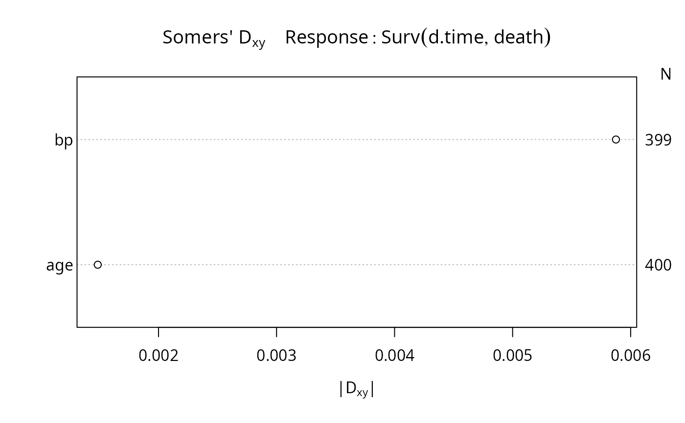
r <- rcorrcens(Surv(d.time, death) ~ age + bp)
r
#> 
#> Somers' Rank Correlation for Censored Data    Response variable:Surv(d.time, death)
#> 
#>         C    Dxy  aDxy    SD    Z     P   n
#> age 0.499 -0.001 0.001 0.037 0.04 0.968 400
#> bp  0.497 -0.006 0.006 0.038 0.15 0.877 399
plot(r)


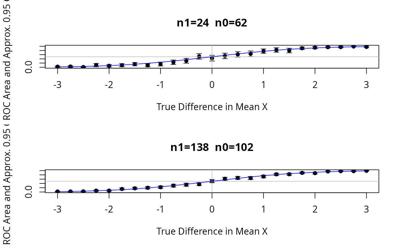
# Show typical 0.95 confidence limits for ROC areas for a sample size
# with 24 events and 62 non-events, for varying population ROC areas
# Repeat for 138 events and 102 non-events
set.seed(8)
par(mfrow=c(2,1))
for(i in 1:2) {
 n1 <- c(24,138)[i]
 n0 <- c(62,102)[i]
 y <- c(rep(0,n0), rep(1,n1))
 deltas <- seq(-3, 3, by=.25)
 C <- se <- deltas
 j <- 0
 for(d in deltas) {
  j <- j + 1
  x <- c(rnorm(n0, 0), rnorm(n1, d))
  w <- rcorr.cens(x, y)
  C[j]  <- w['C Index']
  se[j] <- w['S.D.']/2
 }
 low <- C-1.96*se; hi <- C+1.96*se
 print(cbind(C, low, hi))
 errbar(deltas, C, C+1.96*se, C-1.96*se,
        xlab='True Difference in Mean X',
        ylab='ROC Area and Approx. 0.95 CI')
 title(paste('n1=',n1,'  n0=',n0,sep=''))
 abline(h=.5, v=0, col='gray')
 true <- 1 - pnorm(0, deltas, sqrt(2))
 lines(deltas, true, col='blue')
}
#>            C       low     hi
#>  [1,] 0.0276 -0.001510 0.0566
#>  [2,] 0.0336 -0.000378 0.0676
#>  [3,] 0.0108 -0.004450 0.0260
#>  [4,] 0.1042  0.028482 0.1799
#>  [5,] 0.0679  0.014300 0.1215
#>  [6,] 0.0981  0.026285 0.1700
#>  [7,] 0.1472  0.068762 0.2256
#>  [8,] 0.0927  0.023150 0.1623
#>  [9,] 0.1532  0.060669 0.2458
#> [10,] 0.2386  0.132475 0.3447
#> [11,] 0.3085  0.194064 0.4229
#> [12,] 0.5141  0.385697 0.6425
#> [13,] 0.4335  0.297805 0.5691
#> [14,] 0.5410  0.409413 0.6726
#> [15,] 0.6136  0.486172 0.7410
#> [16,] 0.6418  0.508400 0.7752
#> [17,] 0.7695  0.666004 0.8730
#> [18,] 0.8233  0.718352 0.9282
#> [19,] 0.7977  0.689130 0.9063
#> [20,] 0.9079  0.849626 0.9662
#> [21,] 0.9362  0.882644 0.9897
#> [22,] 0.9577  0.921863 0.9935
#> [23,] 0.9630  0.928010 0.9981
#> [24,] 0.9906  0.978049 1.0031
#> [25,] 0.9718  0.935365 1.0082
#>            C     low     hi
#>  [1,] 0.0220 0.00644 0.0375
#>  [2,] 0.0239 0.00933 0.0385
#>  [3,] 0.0279 0.01162 0.0442
#>  [4,] 0.0635 0.03341 0.0936
#>  [5,] 0.0634 0.03448 0.0924
#>  [6,] 0.1398 0.09424 0.1854
#>  [7,] 0.1701 0.11980 0.2205
#>  [8,] 0.1961 0.14033 0.2518
#>  [9,] 0.2230 0.16465 0.2814
#> [10,] 0.2956 0.22882 0.3624
#> [11,] 0.3382 0.26882 0.4077
#> [12,] 0.3661 0.29566 0.4365
#> [13,] 0.5075 0.43368 0.5812
#> [14,] 0.6153 0.54412 0.6865
#> [15,] 0.6569 0.58852 0.7252
#> [16,] 0.6523 0.58239 0.7222
#> [17,] 0.7237 0.65994 0.7875
#> [18,] 0.8255 0.77347 0.8776
#> [19,] 0.8291 0.77867 0.8796
#> [20,] 0.8939 0.85444 0.9333
#> [21,] 0.8813 0.84016 0.9224
#> [22,] 0.9587 0.93522 0.9821
#> [23,] 0.9716 0.95470 0.9885
#> [24,] 0.9743 0.95601 0.9926
#> [25,] 0.9899 0.98147 0.9983

par(mfrow=c(1,1))