Power and Sample Size for Ordinal Response

popower computes the power for a two-tailed two sample comparison of ordinal outcomes under the proportional odds ordinal logistic model. The power is the same as that of the Wilcoxon test but with ties handled properly. posamsize computes the total sample size needed to achieve a given power. Both functions compute the efficiency of the design compared with a design in which the response variable is continuous. print methods exist for both functions. Any of the input arguments may be vectors, in which case a vector of powers or sample sizes is returned. These functions use the methods of Whitehead (1993).

pomodm is a function that assists in translating odds ratios to differences in mean or median on the original scale.

simPOcuts simulates simple unadjusted two-group comparisons under a PO model to demonstrate the natural sampling variability that causes estimated odds ratios to vary over cutoffs of Y.

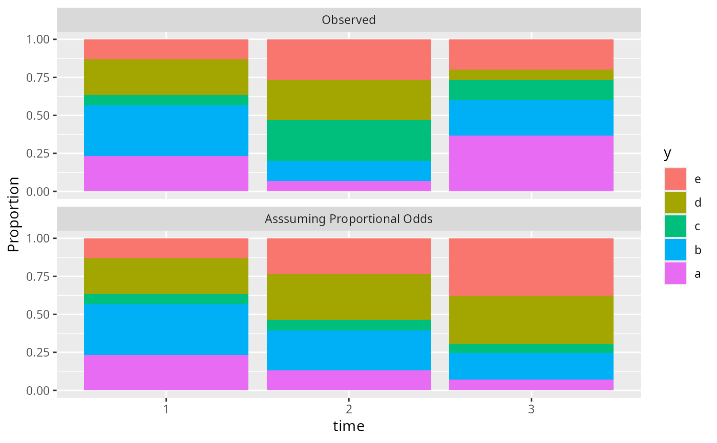
propsPO uses ggplot2 to plot a stacked bar chart of proportions stratified by a grouping variable (and optionally a stratification variable), with an optional additional graph showing what the proportions would be had proportional odds held and an odds ratio was applied to the proportions in a reference group. If the result is passed to ggplotly, customized tooltip hover text will appear.

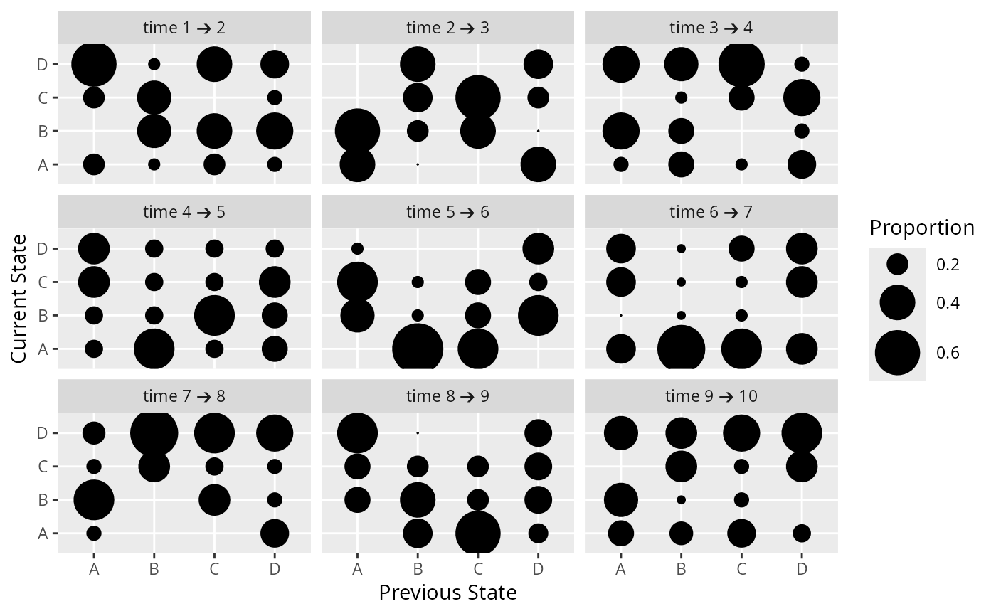
propsTrans uses ggplot2 to plot all successive transition proportions. formula has the state variable on the left hand side, the first right-hand variable is time, and the second right-hand variable is a subject ID variable.\

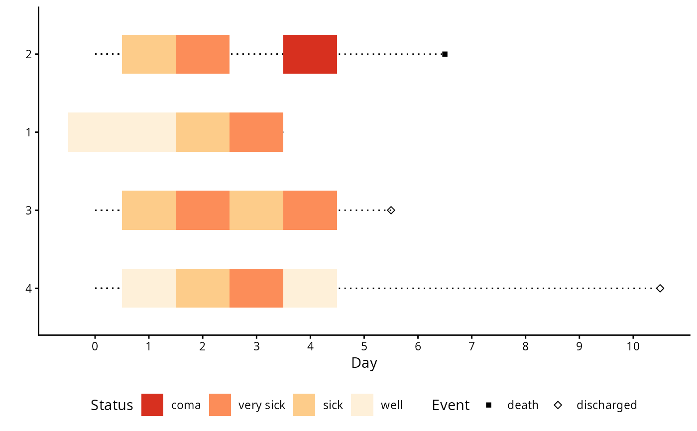
multEventChart uses ggplot2 to plot event charts showing state transitions, account for absorbing states/events. It is based on code written by Lucy D'Agostino McGowan posted at https://livefreeordichotomize.com/posts/2020-05-21-survival-model-detective-1/.

Usage

popower(p, odds.ratio, n, n1, n2, alpha=0.05)
# S3 method for class 'popower'
print(x, ...)
posamsize(p, odds.ratio, fraction=.5, alpha=0.05, power=0.8)
# S3 method for class 'posamsize'
print(x, ...)
pomodm(x=NULL, p, odds.ratio=1)
simPOcuts(n, nsim=10, odds.ratio=1, p)
propsPO(formula, odds.ratio=NULL, ref=NULL, data=NULL, ncol=NULL, nrow=NULL )
propsTrans(formula, data=NULL, labels=NULL, arrow='\u2794',
           maxsize=12, ncol=NULL, nrow=NULL)
multEventChart(formula, data=NULL, absorb=NULL, sortbylast=FALSE,
   colorTitle=label(y), eventTitle='Event',
   palette='OrRd',
   eventSymbols=c(15, 5, 1:4, 6:10),
   timeInc=min(diff(unique(x))/2))

Arguments

p: a vector of marginal cell probabilities which must add up to one. For popower and posamsize, The ith element specifies the probability that a patient will be in response level i, averaged over the two treatment groups. For pomodm and simPOcuts, p is the vector of cell probabilities to be translated under a given odds ratio. For simPOcuts, if p has names, those names are taken as the ordered distinct Y-values. Otherwise Y-values are taken as the integers 1, 2, ... up to the length of p.
odds.ratio: the odds ratio to be able to detect. It doesn't matter which group is in the numerator. For propsPO, odds.ratio is a function of the grouping (right hand side) variable value. The value of the function specifies the odds ratio to apply to the refernce group to get all other group's expected proportions were proportional odds to hold against the first group. Normally the function should return 1.0 when its x argument corresponds to the ref group. For pomodm and simPOcuts is the odds ratio to apply to convert the given cell probabilities.
n: total sample size for popower. You must specify either n or n1 and n2. If you specify n, n1 and n2 are set to n/2. For simPOcuts is a single number equal to the combined sample sizes of two groups.
n1: for popower, the number of subjects in treatment group 1
n2: for popower, the number of subjects in group 2
nsim: number of simulated studies to create by simPOcuts
alpha: type I error
x: an object created by popower or posamsize, or a vector of data values given to pomodm that corresponds to the vector p of probabilities. If x is omitted for pomodm, the odds.ratio will be applied and the new vector of individual probabilities will be returned. Otherwise if x is given to pomodm, a 2-vector with the mean and median x after applying the odds ratio is returned.
fraction: for posamsize, the fraction of subjects that will be allocated to group 1
power: for posamsize, the desired power (default is 0.8)
formula: an R formula expressure for proposPO where the outcome categorical variable is on the left hand side and the grouping variable is on the right. It is assumed that the left hand variable is either already a factor or will have its levels in the right order for an ordinal model when it is converted to factor. For multEventChart the left hand variable is a categorial status variable, the first right hand side variable represents time, and the second right side variable is a unique subject ID. One line is produced per subject.
ref: for propsPO specifies the reference group (value of the right hand side formula variable) to use in computing proportions on which too translate proportions in other groups, under the proportional odds assumption.
data: a data frame or data.table
labels: for propsTrans is an optional character vector corresponding to y=1,2,3,... that is used to construct plotly hovertext as a label attribute in the ggplot2 aesthetic. Used with y is integer on axes but you want long labels in hovertext.
arrow: character to use as the arrow symbol for transitions in propsTrans. The default is the dingbats heavy wide-headed rightwards arror.
nrow,ncol: see facet_wrap
maxsize: maximum symbol size
...: unused
absorb: character vector specifying the subset of levels of the left hand side variable that are absorbing states such as death or hospital discharge
sortbylast: set to TRUE to sort the subjects by the severity of the status at the last time point
colorTitle: label for legend for status
eventTitle: label for legend for absorb
palette: a single character string specifying the scale_fill_brewer color palette
eventSymbols: vector of symbol codes. Default for first two symbols is a solid square and an open diamond.
timeInc: time increment for the x-axis. Default is 1/2 the shortest gap between any two distincttimes in the data.

Value

a list containing power, eff (relative efficiency), and approx.se (approximate standard error of log odds ratio) for popower, or containing n and eff for posamsize.

Author

Frank Harrell
Department of Biostatistics
Vanderbilt University School of Medicine
fh@fharrell.com

References

Whitehead J (1993): Sample size calculations for ordered categorical data. Stat in Med 12:2257–2271.

Julious SA, Campbell MJ (1996): Letter to the Editor. Stat in Med 15: 1065–1066. Shows accuracy of formula for binary response case.

Examples

# For a study of back pain (none, mild, moderate, severe) here are the
# expected proportions (averaged over 2 treatments) that will be in
# each of the 4 categories:


p <- c(.1,.2,.4,.3)
popower(p, 1.2, 1000)   # OR=1.2, total n=1000
#> Power: 0.351 
#> Efficiency of design compared with continuous response: 0.9 
#> Approximate standard error of log odds ratio: 0.116 
#> 
posamsize(p, 1.2)
#> Total sample size: 3148 
#> Efficiency of design compared with continuous response: 0.9 
#> 
popower(p, 1.2, 3148)
#> Power: 0.8 
#> Efficiency of design compared with continuous response: 0.9 
#> Approximate standard error of log odds ratio: 0.0651 
#> 
# If p was the vector of probabilities for group 1, here's how to
# compute the average over the two groups:
# p2   <- pomodm(p=p, odds.ratio=1.2)
# pavg <- (p + p2) / 2

# Compare power to test for proportions for binary case,
# proportion of events in control group of 0.1
p <- 0.1; or <- 0.85; n <- 4000
popower(c(1 - p, p), or, n)    # 0.338
#> Power: 0.338 
#> Efficiency of design compared with continuous response: 0.27 
#> Approximate standard error of log odds ratio: 0.105 
#> 
bpower(p, odds.ratio=or, n=n)  # 0.320
#> Power 
#>  0.32 
# Add more categories, starting with 0.1 in middle
p <- c(.8, .1, .1)
popower(p, or, n)   # 0.543
#> Power: 0.543 
#> Efficiency of design compared with continuous response: 0.486 
#> Approximate standard error of log odds ratio: 0.0786 
#> 
p <- c(.7, .1, .1, .1)
popower(p, or, n)   # 0.67
#> Power: 0.67 
#> Efficiency of design compared with continuous response: 0.654 
#> Approximate standard error of log odds ratio: 0.0677 
#> 
# Continuous scale with final level have prob. 0.1
p <- c(rep(1 / n, 0.9 * n), 0.1)
popower(p, or, n)   # 0.843
#> Power: 0.843 
#> Efficiency of design compared with continuous response: 0.999 
#> Approximate standard error of log odds ratio: 0.0548 
#> 

# Compute the mean and median x after shifting the probability
# distribution by an odds ratio under the proportional odds model
x <- 1 : 5
p <- c(.05, .2, .2, .3, .25)
# For comparison make up a sample that looks like this
X <- rep(1 : 5, 20 * p)
c(mean=mean(X), median=median(X))
#>   mean median 
#>    3.5    4.0 
pomodm(x, p, odds.ratio=1)  # still have to figure out the right median
#>   mean median 
#>   3.50   3.67 
pomodm(x, p, odds.ratio=0.5)
#>   mean median 
#>   3.03   2.95 

# Show variation of odds ratios over possible cutoffs of Y even when PO
# truly holds.  Run 5 simulations for a total sample size of 300.
# The two groups have 150 subjects each.
s <- simPOcuts(300, nsim=5, odds.ratio=2, p=p)
round(s, 2)
#>              y>=2 y>=3 y>=4 y>=5
#> Simulation 1 4.26 1.58 1.40 1.39
#> Simulation 2 4.72 2.28 2.08 1.45
#> Simulation 3 1.63 1.94 2.51 2.47
#> Simulation 4 2.40 2.51 1.81 2.41
#> Simulation 5 1.71 1.79 1.57 1.73

# An ordinal outcome with levels a, b, c, d, e is measured at 3 times
# Show the proportion of values in each outcome category stratified by
# time.  Then compute what the proportions would be had the proportions
# at times 2 and 3 been the proportions at time 1 modified by two odds ratios 

set.seed(1)
d   <- expand.grid(time=1:3, reps=1:30)
d$y <- sample(letters[1:5], nrow(d), replace=TRUE)
propsPO(y ~ time, data=d, odds.ratio=function(time) c(1, 2, 4)[time])
#> Warning: argument is not numeric or logical: returning NA

# To show with plotly, save previous result as object p and then:
# plotly::ggplotly(p, tooltip='label')

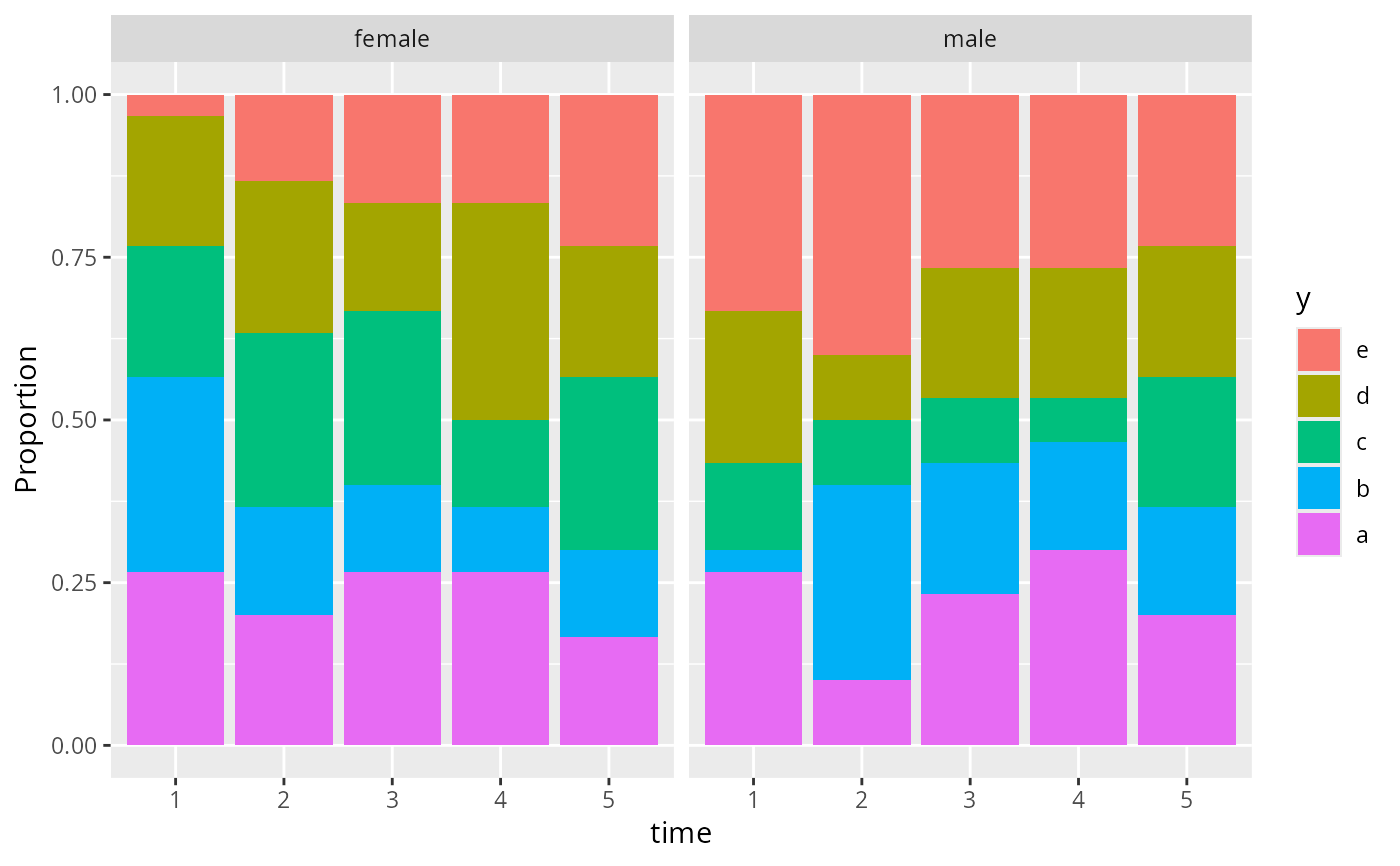
# Add a stratification variable and don't consider an odds ratio
d   <- expand.grid(time=1:5, sex=c('female', 'male'), reps=1:30)
d$y <- sample(letters[1:5], nrow(d), replace=TRUE)
propsPO(y ~ time + sex, data=d)  # may add nrow= or ncol=
#> Warning: argument is not numeric or logical: returning NA
#> Warning: argument is not numeric or logical: returning NA
#> Warning: argument is not numeric or logical: returning NA


# Show all successive transition proportion matrices
d   <- expand.grid(id=1:30, time=1:10)
d$state <- sample(LETTERS[1:4], nrow(d), replace=TRUE)
propsTrans(state ~ time + id, data=d)
#> Warning: argument is not numeric or logical: returning NA
#> Warning: argument is not numeric or logical: returning NA
#> Warning: argument is not numeric or logical: returning NA


pt1 <- data.frame(pt=1, day=0:3,
   status=c('well', 'well', 'sick', 'very sick'))
pt2 <- data.frame(pt=2, day=c(1,2,4,6),
   status=c('sick', 'very sick', 'coma', 'death'))
pt3 <- data.frame(pt=3, day=1:5,
   status=c('sick', 'very sick', 'sick', 'very sick', 'discharged'))
pt4 <- data.frame(pt=4, day=c(1:4, 10),
   status=c('well', 'sick', 'very sick', 'well', 'discharged'))
d <- rbind(pt1, pt2, pt3, pt4)
d$status <- factor(d$status, c('discharged', 'well', 'sick',
                               'very sick', 'coma', 'death'))
label(d$day) <- 'Day'
require(ggplot2)
multEventChart(status ~ day + pt, data=d,
               absorb=c('death', 'discharged'),
               colorTitle='Status', sortbylast=TRUE) +
               theme_classic() +
               theme(legend.position='bottom')
#> Warning: argument is not numeric or logical: returning NA
#> Warning: argument is not numeric or logical: returning NA
#> Warning: argument is not numeric or logical: returning NA