Data and Examples from Stock and Watson (2007)
StockWatson2007.RdThis manual page collects a list of examples from the book. Some solutions might not be exact and the list is certainly not complete. If you have suggestions for improvement (preferably in the form of code), please contact the package maintainer.
References
Stock, J.H. and Watson, M.W. (2007). Introduction to Econometrics, 2nd ed. Boston: Addison Wesley.
See also
CartelStability, CASchools, CigarettesSW,
CollegeDistance, CPSSW04, CPSSW3, CPSSW8,
CPSSW9298, CPSSW9204, CPSSWEducation,
Fatalities, Fertility, Fertility2, FrozenJuice,
GrowthSW, Guns, HealthInsurance, HMDA,
Journals, MASchools, NYSESW, ResumeNames,
SmokeBan, SportsCards, STAR, TeachingRatings,
USMacroSW, USMacroSWM, USMacroSWQ, USSeatBelts,
USStocksSW, WeakInstrument
Examples
###############################
## Current Population Survey ##
###############################
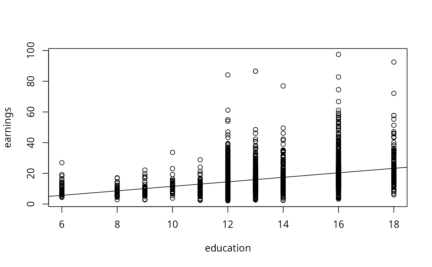
## p. 165
data("CPSSWEducation", package = "AER")
plot(earnings ~ education, data = CPSSWEducation)
fm <- lm(earnings ~ education, data = CPSSWEducation)
coeftest(fm, vcov = sandwich)
#>
#> t test of coefficients:
#>
#> Estimate Std. Error t value Pr(>|t|)
#> (Intercept) -3.134371 0.925571 -3.3864 0.0007174 ***
#> education 1.466925 0.071918 20.3972 < 2.2e-16 ***
#> ---
#> Signif. codes: 0 ‘***’ 0.001 ‘**’ 0.01 ‘*’ 0.05 ‘.’ 0.1 ‘ ’ 1
#>
abline(fm)
 ############################
## California test scores ##
############################
## data and transformations
data("CASchools", package = "AER")
CASchools <- transform(CASchools,
stratio = students/teachers,
score = (math + read)/2
)
## p. 152
fm1 <- lm(score ~ stratio, data = CASchools)
coeftest(fm1, vcov = sandwich)
#>
#> t test of coefficients:
#>
#> Estimate Std. Error t value Pr(>|t|)
#> (Intercept) 698.93295 10.33966 67.597 < 2.2e-16 ***
#> stratio -2.27981 0.51825 -4.399 1.382e-05 ***
#> ---
#> Signif. codes: 0 ‘***’ 0.001 ‘**’ 0.01 ‘*’ 0.05 ‘.’ 0.1 ‘ ’ 1
#>
## p. 159
fm2 <- lm(score ~ I(stratio < 20), data = CASchools)
## p. 199
fm3 <- lm(score ~ stratio + english, data = CASchools)
## p. 224
fm4 <- lm(score ~ stratio + expenditure + english, data = CASchools)
## Table 7.1, p. 242 (numbers refer to columns)
fmc3 <- lm(score ~ stratio + english + lunch, data = CASchools)
fmc4 <- lm(score ~ stratio + english + calworks, data = CASchools)
fmc5 <- lm(score ~ stratio + english + lunch + calworks, data = CASchools)
## Equation 8.2, p. 258
fmquad <- lm(score ~ income + I(income^2), data = CASchools)
## Equation 8.11, p. 266
fmcub <- lm(score ~ income + I(income^2) + I(income^3), data = CASchools)
## Equation 8.23, p. 272
fmloglog <- lm(log(score) ~ log(income), data = CASchools)
## Equation 8.24, p. 274
fmloglin <- lm(log(score) ~ income, data = CASchools)
## Equation 8.26, p. 275
fmlinlogcub <- lm(score ~ log(income) + I(log(income)^2) + I(log(income)^3),
data = CASchools)
## Table 8.3, p. 292 (numbers refer to columns)
fmc2 <- lm(score ~ stratio + english + lunch + log(income), data = CASchools)
fmc7 <- lm(score ~ stratio + I(stratio^2) + I(stratio^3) + english + lunch + log(income),
data = CASchools)
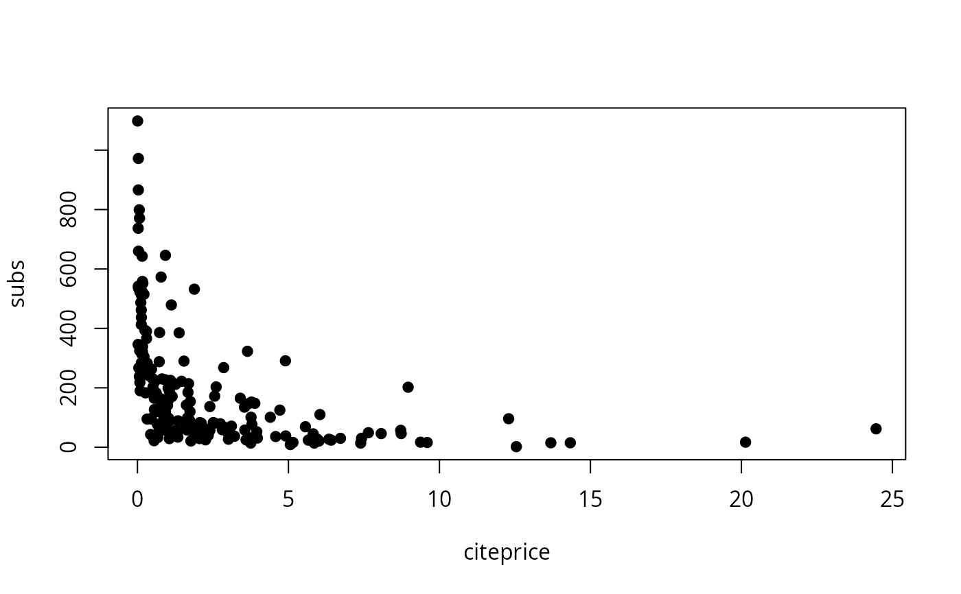
#####################################
## Economics journal Subscriptions ##
#####################################
## data and transformed variables
data("Journals", package = "AER")
journals <- Journals[, c("subs", "price")]
journals$citeprice <- Journals$price/Journals$citations
journals$age <- 2000 - Journals$foundingyear
journals$chars <- Journals$charpp*Journals$pages/10^6
## Figure 8.9 (a) and (b)
plot(subs ~ citeprice, data = journals, pch = 19)
############################
## California test scores ##
############################
## data and transformations
data("CASchools", package = "AER")
CASchools <- transform(CASchools,
stratio = students/teachers,
score = (math + read)/2
)
## p. 152
fm1 <- lm(score ~ stratio, data = CASchools)
coeftest(fm1, vcov = sandwich)
#>
#> t test of coefficients:
#>
#> Estimate Std. Error t value Pr(>|t|)
#> (Intercept) 698.93295 10.33966 67.597 < 2.2e-16 ***
#> stratio -2.27981 0.51825 -4.399 1.382e-05 ***
#> ---
#> Signif. codes: 0 ‘***’ 0.001 ‘**’ 0.01 ‘*’ 0.05 ‘.’ 0.1 ‘ ’ 1
#>
## p. 159
fm2 <- lm(score ~ I(stratio < 20), data = CASchools)
## p. 199
fm3 <- lm(score ~ stratio + english, data = CASchools)
## p. 224
fm4 <- lm(score ~ stratio + expenditure + english, data = CASchools)
## Table 7.1, p. 242 (numbers refer to columns)
fmc3 <- lm(score ~ stratio + english + lunch, data = CASchools)
fmc4 <- lm(score ~ stratio + english + calworks, data = CASchools)
fmc5 <- lm(score ~ stratio + english + lunch + calworks, data = CASchools)
## Equation 8.2, p. 258
fmquad <- lm(score ~ income + I(income^2), data = CASchools)
## Equation 8.11, p. 266
fmcub <- lm(score ~ income + I(income^2) + I(income^3), data = CASchools)
## Equation 8.23, p. 272
fmloglog <- lm(log(score) ~ log(income), data = CASchools)
## Equation 8.24, p. 274
fmloglin <- lm(log(score) ~ income, data = CASchools)
## Equation 8.26, p. 275
fmlinlogcub <- lm(score ~ log(income) + I(log(income)^2) + I(log(income)^3),
data = CASchools)
## Table 8.3, p. 292 (numbers refer to columns)
fmc2 <- lm(score ~ stratio + english + lunch + log(income), data = CASchools)
fmc7 <- lm(score ~ stratio + I(stratio^2) + I(stratio^3) + english + lunch + log(income),
data = CASchools)
#####################################
## Economics journal Subscriptions ##
#####################################
## data and transformed variables
data("Journals", package = "AER")
journals <- Journals[, c("subs", "price")]
journals$citeprice <- Journals$price/Journals$citations
journals$age <- 2000 - Journals$foundingyear
journals$chars <- Journals$charpp*Journals$pages/10^6
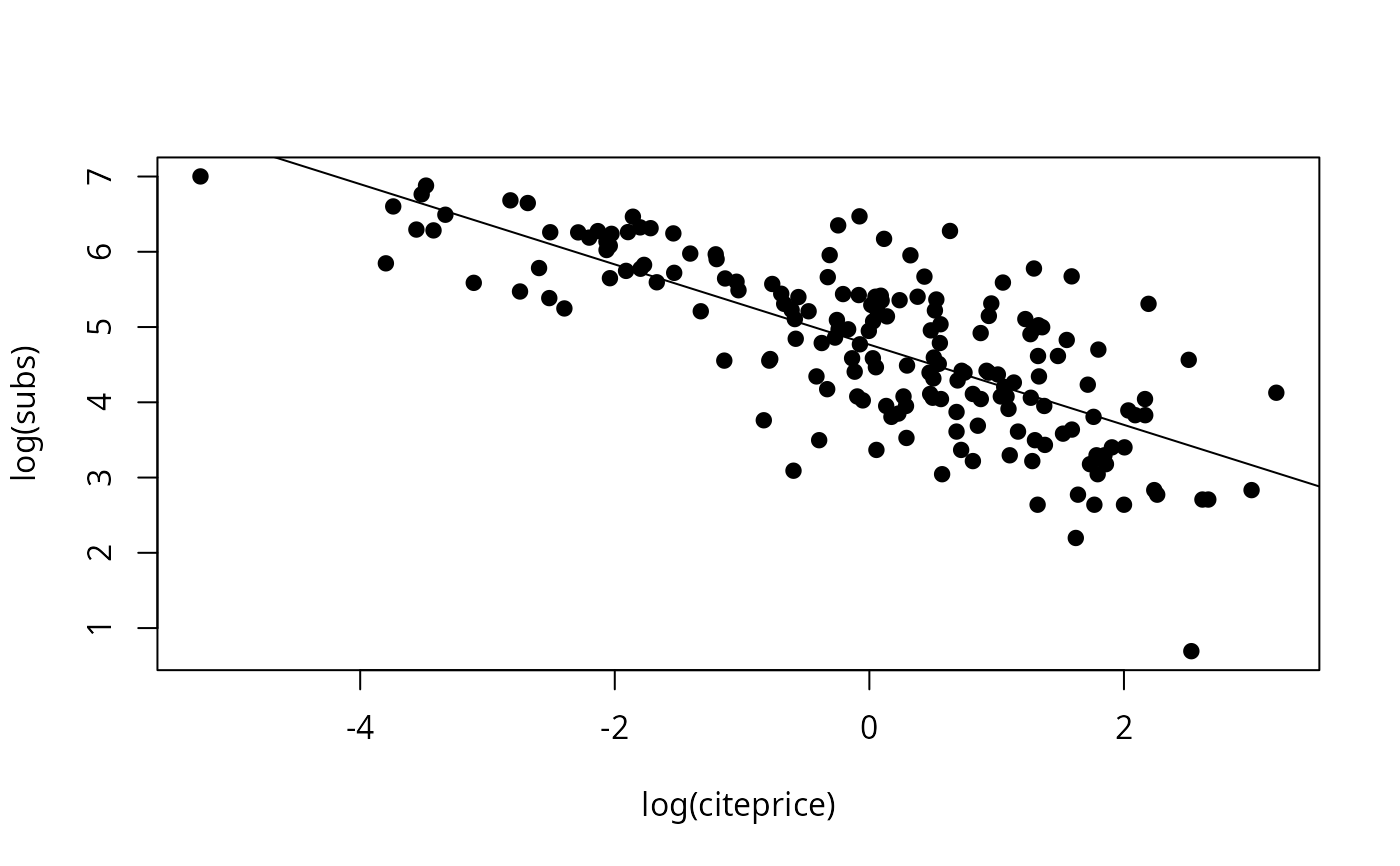
## Figure 8.9 (a) and (b)
plot(subs ~ citeprice, data = journals, pch = 19)
 plot(log(subs) ~ log(citeprice), data = journals, pch = 19)
fm1 <- lm(log(subs) ~ log(citeprice), data = journals)
abline(fm1)
plot(log(subs) ~ log(citeprice), data = journals, pch = 19)
fm1 <- lm(log(subs) ~ log(citeprice), data = journals)
abline(fm1)
 ## Table 8.2, use HC1 for comparability with Stata
fm1 <- lm(subs ~ citeprice, data = log(journals))
fm2 <- lm(subs ~ citeprice + age + chars, data = log(journals))
fm3 <- lm(subs ~ citeprice + I(citeprice^2) + I(citeprice^3) +
age + I(age * citeprice) + chars, data = log(journals))
fm4 <- lm(subs ~ citeprice + age + I(age * citeprice) + chars, data = log(journals))
coeftest(fm1, vcov = vcovHC(fm1, type = "HC1"))
#>
#> t test of coefficients:
#>
#> Estimate Std. Error t value Pr(>|t|)
#> (Intercept) 4.766212 0.055258 86.253 < 2.2e-16 ***
#> citeprice -0.533053 0.033959 -15.697 < 2.2e-16 ***
#> ---
#> Signif. codes: 0 ‘***’ 0.001 ‘**’ 0.01 ‘*’ 0.05 ‘.’ 0.1 ‘ ’ 1
#>
coeftest(fm2, vcov = vcovHC(fm2, type = "HC1"))
#>
#> t test of coefficients:
#>
#> Estimate Std. Error t value Pr(>|t|)
#> (Intercept) 3.206648 0.379725 8.4447 1.102e-14 ***
#> citeprice -0.407718 0.043717 -9.3262 < 2.2e-16 ***
#> age 0.423649 0.119064 3.5581 0.0004801 ***
#> chars 0.205614 0.097751 2.1035 0.0368474 *
#> ---
#> Signif. codes: 0 ‘***’ 0.001 ‘**’ 0.01 ‘*’ 0.05 ‘.’ 0.1 ‘ ’ 1
#>
coeftest(fm3, vcov = vcovHC(fm3, type = "HC1"))
#>
#> t test of coefficients:
#>
#> Estimate Std. Error t value Pr(>|t|)
#> (Intercept) 3.4075956 0.3735992 9.1210 < 2.2e-16 ***
#> citeprice -0.9609365 0.1601349 -6.0008 1.121e-08 ***
#> I(citeprice^2) 0.0165099 0.0254886 0.6477 0.518015
#> I(citeprice^3) 0.0036666 0.0055147 0.6649 0.507008
#> age 0.3730539 0.1176966 3.1696 0.001805 **
#> I(age * citeprice) 0.1557773 0.0518947 3.0018 0.003081 **
#> chars 0.2346178 0.0977318 2.4006 0.017428 *
#> ---
#> Signif. codes: 0 ‘***’ 0.001 ‘**’ 0.01 ‘*’ 0.05 ‘.’ 0.1 ‘ ’ 1
#>
coeftest(fm4, vcov = vcovHC(fm4, type = "HC1"))
#>
#> t test of coefficients:
#>
#> Estimate Std. Error t value Pr(>|t|)
#> (Intercept) 3.433521 0.367471 9.3436 < 2.2e-16 ***
#> citeprice -0.898910 0.144648 -6.2144 3.656e-09 ***
#> age 0.373515 0.117527 3.1781 0.0017529 **
#> I(age * citeprice) 0.140959 0.040199 3.5065 0.0005769 ***
#> chars 0.229466 0.096493 2.3781 0.0184822 *
#> ---
#> Signif. codes: 0 ‘***’ 0.001 ‘**’ 0.01 ‘*’ 0.05 ‘.’ 0.1 ‘ ’ 1
#>
waldtest(fm3, fm4, vcov = vcovHC(fm3, type = "HC1"))
#> Wald test
#>
#> Model 1: subs ~ citeprice + I(citeprice^2) + I(citeprice^3) + age + I(age *
#> citeprice) + chars
#> Model 2: subs ~ citeprice + age + I(age * citeprice) + chars
#> Res.Df Df F Pr(>F)
#> 1 173
#> 2 175 -2 0.249 0.7799
###############################
## Massachusetts test scores ##
###############################
## compare Massachusetts with California
data("MASchools", package = "AER")
data("CASchools", package = "AER")
CASchools <- transform(CASchools,
stratio = students/teachers,
score4 = (math + read)/2
)
## parts of Table 9.1, p. 330
vars <- c("score4", "stratio", "english", "lunch", "income")
cbind(
CA_mean = sapply(CASchools[, vars], mean),
CA_sd = sapply(CASchools[, vars], sd),
MA_mean = sapply(MASchools[, vars], mean),
MA_sd = sapply(MASchools[, vars], sd))
#> CA_mean CA_sd MA_mean MA_sd
#> score4 654.15655 19.053347 709.827273 15.126474
#> stratio 19.64043 1.891812 17.344091 2.276666
#> english 15.76816 18.285927 1.117676 2.900940
#> lunch 44.70524 27.123381 15.315909 15.060068
#> income 15.31659 7.225890 18.746764 5.807637
## Table 9.2, pp. 332--333, numbers refer to columns
MASchools <- transform(MASchools, higheng = english > median(english))
fm1 <- lm(score4 ~ stratio, data = MASchools)
fm2 <- lm(score4 ~ stratio + english + lunch + log(income), data = MASchools)
fm3 <- lm(score4 ~ stratio + english + lunch + income + I(income^2) + I(income^3),
data = MASchools)
fm4 <- lm(score4 ~ stratio + I(stratio^2) + I(stratio^3) + english + lunch +
income + I(income^2) + I(income^3), data = MASchools)
fm5 <- lm(score4 ~ stratio + higheng + I(higheng * stratio) + lunch +
income + I(income^2) + I(income^3), data = MASchools)
fm6 <- lm(score4 ~ stratio + lunch + income + I(income^2) + I(income^3),
data = MASchools)
## for comparability with Stata use HC1 below
coeftest(fm1, vcov = vcovHC(fm1, type = "HC1"))
#>
#> t test of coefficients:
#>
#> Estimate Std. Error t value Pr(>|t|)
#> (Intercept) 739.62113 8.60727 85.9298 < 2.2e-16 ***
#> stratio -1.71781 0.49906 -3.4421 0.000692 ***
#> ---
#> Signif. codes: 0 ‘***’ 0.001 ‘**’ 0.01 ‘*’ 0.05 ‘.’ 0.1 ‘ ’ 1
#>
coeftest(fm2, vcov = vcovHC(fm2, type = "HC1"))
#>
#> t test of coefficients:
#>
#> Estimate Std. Error t value Pr(>|t|)
#> (Intercept) 682.431602 11.497244 59.3561 < 2.2e-16 ***
#> stratio -0.689179 0.269973 -2.5528 0.01138 *
#> english -0.410745 0.306377 -1.3407 0.18145
#> lunch -0.521465 0.077659 -6.7148 1.653e-10 ***
#> log(income) 16.529359 3.145722 5.2546 3.566e-07 ***
#> ---
#> Signif. codes: 0 ‘***’ 0.001 ‘**’ 0.01 ‘*’ 0.05 ‘.’ 0.1 ‘ ’ 1
#>
coeftest(fm3, vcov = vcovHC(fm3, type = "HC1"))
#>
#> t test of coefficients:
#>
#> Estimate Std. Error t value Pr(>|t|)
#> (Intercept) 7.4403e+02 2.1318e+01 34.9016 < 2.2e-16 ***
#> stratio -6.4091e-01 2.6848e-01 -2.3872 0.01785 *
#> english -4.3712e-01 3.0332e-01 -1.4411 0.15103
#> lunch -5.8182e-01 9.7353e-02 -5.9764 9.488e-09 ***
#> income -3.0667e+00 2.3525e+00 -1.3036 0.19379
#> I(income^2) 1.6369e-01 8.5330e-02 1.9183 0.05641 .
#> I(income^3) -2.1793e-03 9.7033e-04 -2.2459 0.02574 *
#> ---
#> Signif. codes: 0 ‘***’ 0.001 ‘**’ 0.01 ‘*’ 0.05 ‘.’ 0.1 ‘ ’ 1
#>
coeftest(fm4, vcov = vcovHC(fm4, type = "HC1"))
#>
#> t test of coefficients:
#>
#> Estimate Std. Error t value Pr(>|t|)
#> (Intercept) 665.4960529 81.3317629 8.1825 2.600e-14 ***
#> stratio 12.4259758 14.0101690 0.8869 0.37613
#> I(stratio^2) -0.6803029 0.7365191 -0.9237 0.35671
#> I(stratio^3) 0.0114737 0.0126663 0.9058 0.36605
#> english -0.4341659 0.2997883 -1.4482 0.14903
#> lunch -0.5872165 0.1040207 -5.6452 5.283e-08 ***
#> income -3.3815370 2.4906830 -1.3577 0.17602
#> I(income^2) 0.1741018 0.0892596 1.9505 0.05244 .
#> I(income^3) -0.0022883 0.0010078 -2.2706 0.02418 *
#> ---
#> Signif. codes: 0 ‘***’ 0.001 ‘**’ 0.01 ‘*’ 0.05 ‘.’ 0.1 ‘ ’ 1
#>
coeftest(fm5, vcov = vcovHC(fm5, type = "HC1"))
#>
#> t test of coefficients:
#>
#> Estimate Std. Error t value Pr(>|t|)
#> (Intercept) 759.9142249 23.2331213 32.7082 < 2.2e-16 ***
#> stratio -1.0176806 0.3703923 -2.7476 0.006521 **
#> highengTRUE -12.5607339 9.7934588 -1.2826 0.201046
#> I(higheng * stratio) 0.7986123 0.5552225 1.4384 0.151805
#> lunch -0.7085098 0.0908442 -7.7992 2.785e-13 ***
#> income -3.8665072 2.4884002 -1.5538 0.121721
#> I(income^2) 0.1841250 0.0898247 2.0498 0.041612 *
#> I(income^3) -0.0023364 0.0010153 -2.3013 0.022349 *
#> ---
#> Signif. codes: 0 ‘***’ 0.001 ‘**’ 0.01 ‘*’ 0.05 ‘.’ 0.1 ‘ ’ 1
#>
coeftest(fm6, vcov = vcovHC(fm6, type = "HC1"))
#>
#> t test of coefficients:
#>
#> Estimate Std. Error t value Pr(>|t|)
#> (Intercept) 7.4736e+02 2.0278e+01 36.8563 < 2e-16 ***
#> stratio -6.7188e-01 2.7128e-01 -2.4767 0.01404 *
#> lunch -6.5308e-01 7.2980e-02 -8.9487 < 2e-16 ***
#> income -3.2180e+00 2.3057e+00 -1.3956 0.16427
#> I(income^2) 1.6479e-01 8.4634e-02 1.9471 0.05284 .
#> I(income^3) -2.1550e-03 9.6995e-04 -2.2218 0.02735 *
#> ---
#> Signif. codes: 0 ‘***’ 0.001 ‘**’ 0.01 ‘*’ 0.05 ‘.’ 0.1 ‘ ’ 1
#>
## Testing exclusion of groups of variables
fm3r <- update(fm3, . ~ . - I(income^2) - I(income^3))
waldtest(fm3, fm3r, vcov = vcovHC(fm3, type = "HC1"))
#> Wald test
#>
#> Model 1: score4 ~ stratio + english + lunch + income + I(income^2) + I(income^3)
#> Model 2: score4 ~ stratio + english + lunch + income
#> Res.Df Df F Pr(>F)
#> 1 213
#> 2 215 -2 7.7448 0.0005664 ***
#> ---
#> Signif. codes: 0 ‘***’ 0.001 ‘**’ 0.01 ‘*’ 0.05 ‘.’ 0.1 ‘ ’ 1
fm4r_str1 <- update(fm4, . ~ . - stratio - I(stratio^2) - I(stratio^3))
waldtest(fm4, fm4r_str1, vcov = vcovHC(fm4, type = "HC1"))
#> Wald test
#>
#> Model 1: score4 ~ stratio + I(stratio^2) + I(stratio^3) + english + lunch +
#> income + I(income^2) + I(income^3)
#> Model 2: score4 ~ english + lunch + income + I(income^2) + I(income^3)
#> Res.Df Df F Pr(>F)
#> 1 211
#> 2 214 -3 2.8565 0.03809 *
#> ---
#> Signif. codes: 0 ‘***’ 0.001 ‘**’ 0.01 ‘*’ 0.05 ‘.’ 0.1 ‘ ’ 1
fm4r_str2 <- update(fm4, . ~ . - I(stratio^2) - I(stratio^3))
waldtest(fm4, fm4r_str2, vcov = vcovHC(fm4, type = "HC1"))
#> Wald test
#>
#> Model 1: score4 ~ stratio + I(stratio^2) + I(stratio^3) + english + lunch +
#> income + I(income^2) + I(income^3)
#> Model 2: score4 ~ stratio + english + lunch + income + I(income^2) + I(income^3)
#> Res.Df Df F Pr(>F)
#> 1 211
#> 2 213 -2 0.4463 0.6406
fm4r_inc <- update(fm4, . ~ . - I(income^2) - I(income^3))
waldtest(fm4, fm4r_inc, vcov = vcovHC(fm4, type = "HC1"))
#> Wald test
#>
#> Model 1: score4 ~ stratio + I(stratio^2) + I(stratio^3) + english + lunch +
#> income + I(income^2) + I(income^3)
#> Model 2: score4 ~ stratio + I(stratio^2) + I(stratio^3) + english + lunch +
#> income
#> Res.Df Df F Pr(>F)
#> 1 211
#> 2 213 -2 7.7487 0.0005657 ***
#> ---
#> Signif. codes: 0 ‘***’ 0.001 ‘**’ 0.01 ‘*’ 0.05 ‘.’ 0.1 ‘ ’ 1
fm5r_str <- update(fm5, . ~ . - stratio - I(higheng * stratio))
waldtest(fm5, fm5r_str, vcov = vcovHC(fm5, type = "HC1"))
#> Wald test
#>
#> Model 1: score4 ~ stratio + higheng + I(higheng * stratio) + lunch + income +
#> I(income^2) + I(income^3)
#> Model 2: score4 ~ higheng + lunch + income + I(income^2) + I(income^3)
#> Res.Df Df F Pr(>F)
#> 1 212
#> 2 214 -2 4.0062 0.0196 *
#> ---
#> Signif. codes: 0 ‘***’ 0.001 ‘**’ 0.01 ‘*’ 0.05 ‘.’ 0.1 ‘ ’ 1
fm5r_inc <- update(fm5, . ~ . - I(income^2) - I(income^3))
waldtest(fm5, fm5r_inc, vcov = vcovHC(fm5, type = "HC1"))
#> Wald test
#>
#> Model 1: score4 ~ stratio + higheng + I(higheng * stratio) + lunch + income +
#> I(income^2) + I(income^3)
#> Model 2: score4 ~ stratio + higheng + I(higheng * stratio) + lunch + income
#> Res.Df Df F Pr(>F)
#> 1 212
#> 2 214 -2 5.8468 0.003375 **
#> ---
#> Signif. codes: 0 ‘***’ 0.001 ‘**’ 0.01 ‘*’ 0.05 ‘.’ 0.1 ‘ ’ 1
fm5r_high <- update(fm5, . ~ . - higheng - I(higheng * stratio))
waldtest(fm5, fm5r_high, vcov = vcovHC(fm5, type = "HC1"))
#> Wald test
#>
#> Model 1: score4 ~ stratio + higheng + I(higheng * stratio) + lunch + income +
#> I(income^2) + I(income^3)
#> Model 2: score4 ~ stratio + lunch + income + I(income^2) + I(income^3)
#> Res.Df Df F Pr(>F)
#> 1 212
#> 2 214 -2 1.5835 0.2077
fm6r_inc <- update(fm6, . ~ . - I(income^2) - I(income^3))
waldtest(fm6, fm6r_inc, vcov = vcovHC(fm6, type = "HC1"))
#> Wald test
#>
#> Model 1: score4 ~ stratio + lunch + income + I(income^2) + I(income^3)
#> Model 2: score4 ~ stratio + lunch + income
#> Res.Df Df F Pr(>F)
#> 1 214
#> 2 216 -2 6.5479 0.001737 **
#> ---
#> Signif. codes: 0 ‘***’ 0.001 ‘**’ 0.01 ‘*’ 0.05 ‘.’ 0.1 ‘ ’ 1
##################################
## Home mortgage disclosure act ##
##################################
## data
data("HMDA", package = "AER")
## 11.1, 11.3, 11.7, 11.8 and 11.10, pp. 387--395
fm1 <- lm(I(as.numeric(deny) - 1) ~ pirat, data = HMDA)
fm2 <- lm(I(as.numeric(deny) - 1) ~ pirat + afam, data = HMDA)
fm3 <- glm(deny ~ pirat, family = binomial(link = "probit"), data = HMDA)
fm4 <- glm(deny ~ pirat + afam, family = binomial(link = "probit"), data = HMDA)
fm5 <- glm(deny ~ pirat + afam, family = binomial(link = "logit"), data = HMDA)
## Table 11.1, p. 401
mean(HMDA$pirat)
#> [1] 0.3308136
mean(HMDA$hirat)
#> [1] 0.2553461
mean(HMDA$lvrat)
#> [1] 0.7377759
mean(as.numeric(HMDA$chist))
#> [1] 2.116387
mean(as.numeric(HMDA$mhist))
#> [1] 1.721008
mean(as.numeric(HMDA$phist)-1)
#> [1] 0.07352941
prop.table(table(HMDA$insurance))
#>
#> no yes
#> 0.97983193 0.02016807
prop.table(table(HMDA$selfemp))
#>
#> no yes
#> 0.8836134 0.1163866
prop.table(table(HMDA$single))
#>
#> no yes
#> 0.6067227 0.3932773
prop.table(table(HMDA$hschool))
#>
#> no yes
#> 0.01638655 0.98361345
mean(HMDA$unemp)
#> [1] 3.774496
prop.table(table(HMDA$condomin))
#>
#> no yes
#> 0.7117647 0.2882353
prop.table(table(HMDA$afam))
#>
#> no yes
#> 0.857563 0.142437
prop.table(table(HMDA$deny))
#>
#> no yes
#> 0.8802521 0.1197479
## Table 11.2, pp. 403--404, numbers refer to columns
HMDA$lvrat <- factor(ifelse(HMDA$lvrat < 0.8, "low",
ifelse(HMDA$lvrat >= 0.8 & HMDA$lvrat <= 0.95, "medium", "high")),
levels = c("low", "medium", "high"))
HMDA$mhist <- as.numeric(HMDA$mhist)
HMDA$chist <- as.numeric(HMDA$chist)
fm1 <- lm(I(as.numeric(deny) - 1) ~ afam + pirat + hirat + lvrat + chist + mhist +
phist + insurance + selfemp, data = HMDA)
fm2 <- glm(deny ~ afam + pirat + hirat + lvrat + chist + mhist + phist + insurance +
selfemp, family = binomial, data = HMDA)
fm3 <- glm(deny ~ afam + pirat + hirat + lvrat + chist + mhist + phist + insurance +
selfemp, family = binomial(link = "probit"), data = HMDA)
fm4 <- glm(deny ~ afam + pirat + hirat + lvrat + chist + mhist + phist + insurance +
selfemp + single + hschool + unemp, family = binomial(link = "probit"), data = HMDA)
fm5 <- glm(deny ~ afam + pirat + hirat + lvrat + chist + mhist + phist + insurance +
selfemp + single + hschool + unemp + condomin +
I(mhist==3) + I(mhist==4) + I(chist==3) + I(chist==4) + I(chist==5) + I(chist==6),
family = binomial(link = "probit"), data = HMDA)
fm6 <- glm(deny ~ afam * (pirat + hirat) + lvrat + chist + mhist + phist + insurance +
selfemp + single + hschool + unemp, family = binomial(link = "probit"), data = HMDA)
coeftest(fm1, vcov = sandwich)
#>
#> t test of coefficients:
#>
#> Estimate Std. Error t value Pr(>|t|)
#> (Intercept) -0.1829933 0.0276089 -6.6281 4.197e-11 ***
#> afamyes 0.0836967 0.0225101 3.7182 0.0002053 ***
#> pirat 0.4487963 0.1133333 3.9600 7.717e-05 ***
#> hirat -0.0480227 0.1093055 -0.4393 0.6604528
#> lvratmedium 0.0314498 0.0127097 2.4745 0.0134125 *
#> lvrathigh 0.1890511 0.0500520 3.7771 0.0001626 ***
#> chist 0.0307716 0.0045737 6.7279 2.150e-11 ***
#> mhist 0.0209104 0.0112637 1.8565 0.0635134 .
#> phistyes 0.1970876 0.0348005 5.6634 1.664e-08 ***
#> insuranceyes 0.7018841 0.0450008 15.5972 < 2.2e-16 ***
#> selfempyes 0.0598438 0.0204759 2.9227 0.0035035 **
#> ---
#> Signif. codes: 0 ‘***’ 0.001 ‘**’ 0.01 ‘*’ 0.05 ‘.’ 0.1 ‘ ’ 1
#>
fm4r <- update(fm4, . ~ . - single - hschool - unemp)
waldtest(fm4, fm4r, vcov = sandwich)
#> Wald test
#>
#> Model 1: deny ~ afam + pirat + hirat + lvrat + chist + mhist + phist +
#> insurance + selfemp + single + hschool + unemp
#> Model 2: deny ~ afam + pirat + hirat + lvrat + chist + mhist + phist +
#> insurance + selfemp
#> Res.Df Df F Pr(>F)
#> 1 2366
#> 2 2369 -3 5.9463 0.0004893 ***
#> ---
#> Signif. codes: 0 ‘***’ 0.001 ‘**’ 0.01 ‘*’ 0.05 ‘.’ 0.1 ‘ ’ 1
fm5r <- update(fm5, . ~ . - single - hschool - unemp)
waldtest(fm5, fm5r, vcov = sandwich)
#> Wald test
#>
#> Model 1: deny ~ afam + pirat + hirat + lvrat + chist + mhist + phist +
#> insurance + selfemp + single + hschool + unemp + condomin +
#> I(mhist == 3) + I(mhist == 4) + I(chist == 3) + I(chist ==
#> 4) + I(chist == 5) + I(chist == 6)
#> Model 2: deny ~ afam + pirat + hirat + lvrat + chist + mhist + phist +
#> insurance + selfemp + condomin + I(mhist == 3) + I(mhist ==
#> 4) + I(chist == 3) + I(chist == 4) + I(chist == 5) + I(chist ==
#> 6)
#> Res.Df Df F Pr(>F)
#> 1 2359
#> 2 2362 -3 5.1601 0.001482 **
#> ---
#> Signif. codes: 0 ‘***’ 0.001 ‘**’ 0.01 ‘*’ 0.05 ‘.’ 0.1 ‘ ’ 1
fm6r <- update(fm6, . ~ . - single - hschool - unemp)
waldtest(fm6, fm6r, vcov = sandwich)
#> Wald test
#>
#> Model 1: deny ~ afam * (pirat + hirat) + lvrat + chist + mhist + phist +
#> insurance + selfemp + single + hschool + unemp
#> Model 2: deny ~ afam + pirat + hirat + lvrat + chist + mhist + phist +
#> insurance + selfemp + afam:pirat + afam:hirat
#> Res.Df Df F Pr(>F)
#> 1 2364
#> 2 2367 -3 5.8876 0.0005316 ***
#> ---
#> Signif. codes: 0 ‘***’ 0.001 ‘**’ 0.01 ‘*’ 0.05 ‘.’ 0.1 ‘ ’ 1
fm5r2 <- update(fm5, . ~ . - I(mhist==3) - I(mhist==4) - I(chist==3) - I(chist==4) -
I(chist==5) - I(chist==6))
waldtest(fm5, fm5r2, vcov = sandwich)
#> Wald test
#>
#> Model 1: deny ~ afam + pirat + hirat + lvrat + chist + mhist + phist +
#> insurance + selfemp + single + hschool + unemp + condomin +
#> I(mhist == 3) + I(mhist == 4) + I(chist == 3) + I(chist ==
#> 4) + I(chist == 5) + I(chist == 6)
#> Model 2: deny ~ afam + pirat + hirat + lvrat + chist + mhist + phist +
#> insurance + selfemp + single + hschool + unemp + condomin
#> Res.Df Df F Pr(>F)
#> 1 2359
#> 2 2365 -6 1.2305 0.2873
fm6r2 <- update(fm6, . ~ . - afam * (pirat + hirat) + pirat + hirat)
waldtest(fm6, fm6r2, vcov = sandwich)
#> Wald test
#>
#> Model 1: deny ~ afam * (pirat + hirat) + lvrat + chist + mhist + phist +
#> insurance + selfemp + single + hschool + unemp
#> Model 2: deny ~ lvrat + chist + mhist + phist + insurance + selfemp +
#> single + hschool + unemp + pirat + hirat
#> Res.Df Df F Pr(>F)
#> 1 2364
#> 2 2367 -3 4.9217 0.00207 **
#> ---
#> Signif. codes: 0 ‘***’ 0.001 ‘**’ 0.01 ‘*’ 0.05 ‘.’ 0.1 ‘ ’ 1
fm6r3 <- update(fm6, . ~ . - afam * (pirat + hirat) + pirat + hirat + afam)
waldtest(fm6, fm6r3, vcov = sandwich)
#> Wald test
#>
#> Model 1: deny ~ afam * (pirat + hirat) + lvrat + chist + mhist + phist +
#> insurance + selfemp + single + hschool + unemp
#> Model 2: deny ~ lvrat + chist + mhist + phist + insurance + selfemp +
#> single + hschool + unemp + pirat + hirat + afam
#> Res.Df Df F Pr(>F)
#> 1 2364
#> 2 2366 -2 0.2634 0.7685
#########################################################
## Shooting down the "More Guns Less Crime" hypothesis ##
#########################################################
## data
data("Guns", package = "AER")
## Empirical Exercise 10.1
fm1 <- lm(log(violent) ~ law, data = Guns)
fm2 <- lm(log(violent) ~ law + prisoners + density + income +
population + afam + cauc + male, data = Guns)
fm3 <- lm(log(violent) ~ law + prisoners + density + income +
population + afam + cauc + male + state, data = Guns)
fm4 <- lm(log(violent) ~ law + prisoners + density + income +
population + afam + cauc + male + state + year, data = Guns)
coeftest(fm1, vcov = sandwich)
#>
#> t test of coefficients:
#>
#> Estimate Std. Error t value Pr(>|t|)
#> (Intercept) 6.134919 0.019287 318.078 < 2.2e-16 ***
#> lawyes -0.442965 0.047488 -9.328 < 2.2e-16 ***
#> ---
#> Signif. codes: 0 ‘***’ 0.001 ‘**’ 0.01 ‘*’ 0.05 ‘.’ 0.1 ‘ ’ 1
#>
coeftest(fm2, vcov = sandwich)
#>
#> t test of coefficients:
#>
#> Estimate Std. Error t value Pr(>|t|)
#> (Intercept) 2.9817e+00 6.0668e-01 4.9149 1.016e-06 ***
#> lawyes -3.6839e-01 3.4654e-02 -10.6304 < 2.2e-16 ***
#> prisoners 1.6126e-03 1.8000e-04 8.9591 < 2.2e-16 ***
#> density 2.6688e-02 1.4294e-02 1.8671 0.062142 .
#> income 1.2051e-06 7.2498e-06 0.1662 0.868007
#> population 4.2710e-02 3.1345e-03 13.6255 < 2.2e-16 ***
#> afam 8.0853e-02 1.9916e-02 4.0598 5.241e-05 ***
#> cauc 3.1200e-02 9.6897e-03 3.2200 0.001317 **
#> male 8.8709e-03 1.2014e-02 0.7384 0.460435
#> ---
#> Signif. codes: 0 ‘***’ 0.001 ‘**’ 0.01 ‘*’ 0.05 ‘.’ 0.1 ‘ ’ 1
#>
printCoefmat(coeftest(fm3, vcov = sandwich)[1:9,])
#> Estimate Std. Error t value Pr(>|t|)
#> (Intercept) 4.0368e+00 3.7479e-01 10.7708 < 2.2e-16 ***
#> lawyes -4.6141e-02 1.9435e-02 -2.3741 0.01776 *
#> prisoners -7.1008e-05 9.4831e-05 -0.7488 0.45414
#> density -1.7229e-01 1.0221e-01 -1.6857 0.09213 .
#> income -9.2037e-06 6.5619e-06 -1.4026 0.16102
#> population 1.1525e-02 9.4572e-03 1.2186 0.22325
#> afam 1.0428e-01 1.6133e-02 6.4636 1.526e-10 ***
#> cauc 4.0861e-02 5.2487e-03 7.7850 1.585e-14 ***
#> male -5.0273e-02 7.5923e-03 -6.6215 5.518e-11 ***
#> ---
#> Signif. codes: 0 ‘***’ 0.001 ‘**’ 0.01 ‘*’ 0.05 ‘.’ 0.1 ‘ ’ 1
printCoefmat(coeftest(fm4, vcov = sandwich)[1:9,])
#> Estimate Std. Error t value Pr(>|t|)
#> (Intercept) 3.9720e+00 4.3322e-01 9.1685 < 2.2e-16 ***
#> lawyes -2.7994e-02 1.8692e-02 -1.4976 0.1345
#> prisoners 7.5994e-05 8.0008e-05 0.9498 0.3424
#> density -9.1555e-02 6.2588e-02 -1.4628 0.1438
#> income 9.5859e-07 6.9440e-06 0.1380 0.8902
#> population -4.7545e-03 6.4673e-03 -0.7351 0.4624
#> afam 2.9186e-02 2.0298e-02 1.4379 0.1507
#> cauc 9.2500e-03 8.2188e-03 1.1255 0.2606
#> male 7.3326e-02 1.8116e-02 4.0475 5.542e-05 ***
#> ---
#> Signif. codes: 0 ‘***’ 0.001 ‘**’ 0.01 ‘*’ 0.05 ‘.’ 0.1 ‘ ’ 1
###########################
## US traffic fatalities ##
###########################
## data from Stock and Watson (2007)
data("Fatalities", package = "AER")
Fatalities <- transform(Fatalities,
## fatality rate (number of traffic deaths per 10,000 people living in that state in that year)
frate = fatal/pop * 10000,
## add discretized version of minimum legal drinking age
drinkagec = relevel(cut(drinkage, breaks = 18:22, include.lowest = TRUE, right = FALSE), ref = 4),
## any punishment?
punish = factor(jail == "yes" | service == "yes", labels = c("no", "yes"))
)
## plm package
library("plm")
## for comparability with Stata we use HC1 below
## p. 351, Eq. (10.2)
f1982 <- subset(Fatalities, year == "1982")
fm_1982 <- lm(frate ~ beertax, data = f1982)
coeftest(fm_1982, vcov = vcovHC(fm_1982, type = "HC1"))
#>
#> t test of coefficients:
#>
#> Estimate Std. Error t value Pr(>|t|)
#> (Intercept) 2.01038 0.14957 13.4408 <2e-16 ***
#> beertax 0.14846 0.13261 1.1196 0.2687
#> ---
#> Signif. codes: 0 ‘***’ 0.001 ‘**’ 0.01 ‘*’ 0.05 ‘.’ 0.1 ‘ ’ 1
#>
## p. 353, Eq. (10.3)
f1988 <- subset(Fatalities, year == "1988")
fm_1988 <- lm(frate ~ beertax, data = f1988)
coeftest(fm_1988, vcov = vcovHC(fm_1988, type = "HC1"))
#>
#> t test of coefficients:
#>
#> Estimate Std. Error t value Pr(>|t|)
#> (Intercept) 1.85907 0.11461 16.2205 < 2.2e-16 ***
#> beertax 0.43875 0.12786 3.4314 0.001279 **
#> ---
#> Signif. codes: 0 ‘***’ 0.001 ‘**’ 0.01 ‘*’ 0.05 ‘.’ 0.1 ‘ ’ 1
#>
## pp. 355, Eq. (10.8)
fm_diff <- lm(I(f1988$frate - f1982$frate) ~ I(f1988$beertax - f1982$beertax))
coeftest(fm_diff, vcov = vcovHC(fm_diff, type = "HC1"))
#>
#> t test of coefficients:
#>
#> Estimate Std. Error t value Pr(>|t|)
#> (Intercept) -0.072037 0.065355 -1.1022 0.276091
#> I(f1988$beertax - f1982$beertax) -1.040973 0.355006 -2.9323 0.005229 **
#> ---
#> Signif. codes: 0 ‘***’ 0.001 ‘**’ 0.01 ‘*’ 0.05 ‘.’ 0.1 ‘ ’ 1
#>
## pp. 360, Eq. (10.15)
## (1) via formula
fm_sfe <- lm(frate ~ beertax + state - 1, data = Fatalities)
## (2) by hand
fat <- with(Fatalities,
data.frame(frates = frate - ave(frate, state),
beertaxs = beertax - ave(beertax, state)))
fm_sfe2 <- lm(frates ~ beertaxs - 1, data = fat)
## (3) via plm()
fm_sfe3 <- plm(frate ~ beertax, data = Fatalities,
index = c("state", "year"), model = "within")
coeftest(fm_sfe, vcov = vcovHC(fm_sfe, type = "HC1"))[1,]
#> Estimate Std. Error t value Pr(>|t|)
#> -0.655873722 0.203279719 -3.226459220 0.001398372
## uses different df in sd and p-value
coeftest(fm_sfe2, vcov = vcovHC(fm_sfe2, type = "HC1"))[1,]
#> Estimate Std. Error t value Pr(>|t|)
#> -0.655873722 0.188153627 -3.485841496 0.000555894
## uses different df in p-value
coeftest(fm_sfe3, vcov = vcovHC(fm_sfe3, type = "HC1", method = "white1"))[1,]
#> Estimate Std. Error t value Pr(>|t|)
#> -0.6558737222 0.1881536274 -3.4858414958 0.0005673213
## pp. 363, Eq. (10.21)
## via lm()
fm_stfe <- lm(frate ~ beertax + state + year - 1, data = Fatalities)
coeftest(fm_stfe, vcov = vcovHC(fm_stfe, type = "HC1"))[1,]
#> Estimate Std. Error t value Pr(>|t|)
#> -0.6399800 0.2547149 -2.5125346 0.0125470
## via plm()
fm_stfe2 <- plm(frate ~ beertax, data = Fatalities,
index = c("state", "year"), model = "within", effect = "twoways")
coeftest(fm_stfe2, vcov = vcovHC) ## different
#>
#> t test of coefficients:
#>
#> Estimate Std. Error t value Pr(>|t|)
#> beertax -0.63998 0.34963 -1.8305 0.06824 .
#> ---
#> Signif. codes: 0 ‘***’ 0.001 ‘**’ 0.01 ‘*’ 0.05 ‘.’ 0.1 ‘ ’ 1
#>
## p. 368, Table 10.1, numbers refer to cols.
fm1 <- plm(frate ~ beertax, data = Fatalities, index = c("state", "year"),
model = "pooling")
fm2 <- plm(frate ~ beertax, data = Fatalities, index = c("state", "year"),
model = "within")
fm3 <- plm(frate ~ beertax, data = Fatalities, index = c("state", "year"),
model = "within", effect = "twoways")
fm4 <- plm(frate ~ beertax + drinkagec + jail + service + miles + unemp + log(income),
data = Fatalities, index = c("state", "year"), model = "within", effect = "twoways")
fm5 <- plm(frate ~ beertax + drinkagec + jail + service + miles,
data = Fatalities, index = c("state", "year"), model = "within", effect = "twoways")
fm6 <- plm(frate ~ beertax + drinkage + punish + miles + unemp + log(income),
data = Fatalities, index = c("state", "year"), model = "within", effect = "twoways")
fm7 <- plm(frate ~ beertax + drinkagec + jail + service + miles + unemp + log(income),
data = Fatalities, index = c("state", "year"), model = "within", effect = "twoways")
## summaries not too close, s.e.s generally too small
coeftest(fm1, vcov = vcovHC)
#>
#> t test of coefficients:
#>
#> Estimate Std. Error t value Pr(>|t|)
#> (Intercept) 1.85331 0.11710 15.8263 < 2.2e-16 ***
#> beertax 0.36461 0.11826 3.0832 0.002218 **
#> ---
#> Signif. codes: 0 ‘***’ 0.001 ‘**’ 0.01 ‘*’ 0.05 ‘.’ 0.1 ‘ ’ 1
#>
coeftest(fm2, vcov = vcovHC)
#>
#> t test of coefficients:
#>
#> Estimate Std. Error t value Pr(>|t|)
#> beertax -0.65587 0.28837 -2.2744 0.02368 *
#> ---
#> Signif. codes: 0 ‘***’ 0.001 ‘**’ 0.01 ‘*’ 0.05 ‘.’ 0.1 ‘ ’ 1
#>
coeftest(fm3, vcov = vcovHC)
#>
#> t test of coefficients:
#>
#> Estimate Std. Error t value Pr(>|t|)
#> beertax -0.63998 0.34963 -1.8305 0.06824 .
#> ---
#> Signif. codes: 0 ‘***’ 0.001 ‘**’ 0.01 ‘*’ 0.05 ‘.’ 0.1 ‘ ’ 1
#>
coeftest(fm4, vcov = vcovHC)
#>
#> t test of coefficients:
#>
#> Estimate Std. Error t value Pr(>|t|)
#> beertax -4.4895e-01 2.8850e-01 -1.5562 0.120828
#> drinkagec[18,19) 2.8149e-02 6.8014e-02 0.4139 0.679299
#> drinkagec[19,20) -1.8550e-02 4.8162e-02 -0.3852 0.700416
#> drinkagec[20,21) 3.1375e-02 4.8744e-02 0.6437 0.520323
#> jailyes 1.3058e-02 1.6115e-02 0.8103 0.418458
#> serviceyes 3.3446e-02 1.2873e-01 0.2598 0.795197
#> miles 8.2275e-06 6.6313e-06 1.2407 0.215785
#> unemp -6.3111e-02 1.2615e-02 -5.0028 1.015e-06 ***
#> log(income) 1.8146e+00 6.1659e-01 2.9429 0.003532 **
#> ---
#> Signif. codes: 0 ‘***’ 0.001 ‘**’ 0.01 ‘*’ 0.05 ‘.’ 0.1 ‘ ’ 1
#>
coeftest(fm5, vcov = vcovHC)
#>
#> t test of coefficients:
#>
#> Estimate Std. Error t value Pr(>|t|)
#> beertax -7.0442e-01 3.3804e-01 -2.0838 0.03810 *
#> drinkagec[18,19) -1.1360e-02 8.0764e-02 -0.1407 0.88825
#> drinkagec[19,20) -7.8033e-02 6.5591e-02 -1.1897 0.23520
#> drinkagec[20,21) -1.0224e-01 5.4695e-02 -1.8692 0.06266 .
#> jailyes -2.5965e-02 1.8624e-02 -1.3942 0.16439
#> serviceyes 1.4690e-01 1.3970e-01 1.0515 0.29395
#> miles 1.7372e-05 1.0221e-05 1.6996 0.09033 .
#> ---
#> Signif. codes: 0 ‘***’ 0.001 ‘**’ 0.01 ‘*’ 0.05 ‘.’ 0.1 ‘ ’ 1
#>
coeftest(fm6, vcov = vcovHC)
#>
#> t test of coefficients:
#>
#> Estimate Std. Error t value Pr(>|t|)
#> beertax -4.5647e-01 2.9809e-01 -1.5313 0.126845
#> drinkage -2.1567e-03 2.0908e-02 -0.1032 0.917916
#> punishyes 3.8981e-02 1.0023e-01 0.3889 0.697636
#> miles 8.9787e-06 6.8958e-06 1.3020 0.193991
#> unemp -6.2694e-02 1.2854e-02 -4.8776 1.82e-06 ***
#> log(income) 1.7864e+00 6.2511e-01 2.8578 0.004592 **
#> ---
#> Signif. codes: 0 ‘***’ 0.001 ‘**’ 0.01 ‘*’ 0.05 ‘.’ 0.1 ‘ ’ 1
#>
coeftest(fm7, vcov = vcovHC)
#>
#> t test of coefficients:
#>
#> Estimate Std. Error t value Pr(>|t|)
#> beertax -4.4895e-01 2.8850e-01 -1.5562 0.120828
#> drinkagec[18,19) 2.8149e-02 6.8014e-02 0.4139 0.679299
#> drinkagec[19,20) -1.8550e-02 4.8162e-02 -0.3852 0.700416
#> drinkagec[20,21) 3.1375e-02 4.8744e-02 0.6437 0.520323
#> jailyes 1.3058e-02 1.6115e-02 0.8103 0.418458
#> serviceyes 3.3446e-02 1.2873e-01 0.2598 0.795197
#> miles 8.2275e-06 6.6313e-06 1.2407 0.215785
#> unemp -6.3111e-02 1.2615e-02 -5.0028 1.015e-06 ***
#> log(income) 1.8146e+00 6.1659e-01 2.9429 0.003532 **
#> ---
#> Signif. codes: 0 ‘***’ 0.001 ‘**’ 0.01 ‘*’ 0.05 ‘.’ 0.1 ‘ ’ 1
#>
######################################
## Cigarette consumption panel data ##
######################################
## data and transformations
data("CigarettesSW", package = "AER")
CigarettesSW <- transform(CigarettesSW,
rprice = price/cpi,
rincome = income/population/cpi,
rtax = tax/cpi,
rtdiff = (taxs - tax)/cpi
)
c1985 <- subset(CigarettesSW, year == "1985")
c1995 <- subset(CigarettesSW, year == "1995")
## convenience function: HC1 covariances
hc1 <- function(x) vcovHC(x, type = "HC1")
## Equations 12.9--12.11
fm_s1 <- lm(log(rprice) ~ rtdiff, data = c1995)
coeftest(fm_s1, vcov = hc1)
#>
#> t test of coefficients:
#>
#> Estimate Std. Error t value Pr(>|t|)
#> (Intercept) 4.6165463 0.0289177 159.6444 < 2.2e-16 ***
#> rtdiff 0.0307289 0.0048354 6.3549 8.489e-08 ***
#> ---
#> Signif. codes: 0 ‘***’ 0.001 ‘**’ 0.01 ‘*’ 0.05 ‘.’ 0.1 ‘ ’ 1
#>
fm_s2 <- lm(log(packs) ~ fitted(fm_s1), data = c1995)
fm_ivreg <- ivreg(log(packs) ~ log(rprice) | rtdiff, data = c1995)
coeftest(fm_ivreg, vcov = hc1)
#>
#> t test of coefficients:
#>
#> Estimate Std. Error t value Pr(>|t|)
#> (Intercept) 9.71988 1.52832 6.3598 8.346e-08 ***
#> log(rprice) -1.08359 0.31892 -3.3977 0.001411 **
#> ---
#> Signif. codes: 0 ‘***’ 0.001 ‘**’ 0.01 ‘*’ 0.05 ‘.’ 0.1 ‘ ’ 1
#>
## Equation 12.15
fm_ivreg2 <- ivreg(log(packs) ~ log(rprice) + log(rincome) | log(rincome) + rtdiff, data = c1995)
coeftest(fm_ivreg2, vcov = hc1)
#>
#> t test of coefficients:
#>
#> Estimate Std. Error t value Pr(>|t|)
#> (Intercept) 9.43066 1.25939 7.4883 1.935e-09 ***
#> log(rprice) -1.14338 0.37230 -3.0711 0.003611 **
#> log(rincome) 0.21452 0.31175 0.6881 0.494917
#> ---
#> Signif. codes: 0 ‘***’ 0.001 ‘**’ 0.01 ‘*’ 0.05 ‘.’ 0.1 ‘ ’ 1
#>
## Equation 12.16
fm_ivreg3 <- ivreg(log(packs) ~ log(rprice) + log(rincome) | log(rincome) + rtdiff + rtax,
data = c1995)
coeftest(fm_ivreg3, vcov = hc1)
#>
#> t test of coefficients:
#>
#> Estimate Std. Error t value Pr(>|t|)
#> (Intercept) 9.89496 0.95922 10.3157 1.947e-13 ***
#> log(rprice) -1.27742 0.24961 -5.1177 6.211e-06 ***
#> log(rincome) 0.28040 0.25389 1.1044 0.2753
#> ---
#> Signif. codes: 0 ‘***’ 0.001 ‘**’ 0.01 ‘*’ 0.05 ‘.’ 0.1 ‘ ’ 1
#>
## Table 12.1, p. 448
ydiff <- log(c1995$packs) - log(c1985$packs)
pricediff <- log(c1995$price/c1995$cpi) - log(c1985$price/c1985$cpi)
incdiff <- log(c1995$income/c1995$population/c1995$cpi) -
log(c1985$income/c1985$population/c1985$cpi)
taxsdiff <- (c1995$taxs - c1995$tax)/c1995$cpi - (c1985$taxs - c1985$tax)/c1985$cpi
taxdiff <- c1995$tax/c1995$cpi - c1985$tax/c1985$cpi
fm_diff1 <- ivreg(ydiff ~ pricediff + incdiff | incdiff + taxsdiff)
fm_diff2 <- ivreg(ydiff ~ pricediff + incdiff | incdiff + taxdiff)
fm_diff3 <- ivreg(ydiff ~ pricediff + incdiff | incdiff + taxsdiff + taxdiff)
coeftest(fm_diff1, vcov = hc1)
#>
#> t test of coefficients:
#>
#> Estimate Std. Error t value Pr(>|t|)
#> (Intercept) -0.117962 0.068217 -1.7292 0.09062 .
#> pricediff -0.938014 0.207502 -4.5205 4.454e-05 ***
#> incdiff 0.525970 0.339494 1.5493 0.12832
#> ---
#> Signif. codes: 0 ‘***’ 0.001 ‘**’ 0.01 ‘*’ 0.05 ‘.’ 0.1 ‘ ’ 1
#>
coeftest(fm_diff2, vcov = hc1)
#>
#> t test of coefficients:
#>
#> Estimate Std. Error t value Pr(>|t|)
#> (Intercept) -0.017049 0.067217 -0.2536 0.8009
#> pricediff -1.342515 0.228661 -5.8712 4.848e-07 ***
#> incdiff 0.428146 0.298718 1.4333 0.1587
#> ---
#> Signif. codes: 0 ‘***’ 0.001 ‘**’ 0.01 ‘*’ 0.05 ‘.’ 0.1 ‘ ’ 1
#>
coeftest(fm_diff3, vcov = hc1)
#>
#> t test of coefficients:
#>
#> Estimate Std. Error t value Pr(>|t|)
#> (Intercept) -0.052003 0.062488 -0.8322 0.4097
#> pricediff -1.202403 0.196943 -6.1053 2.178e-07 ***
#> incdiff 0.462030 0.309341 1.4936 0.1423
#> ---
#> Signif. codes: 0 ‘***’ 0.001 ‘**’ 0.01 ‘*’ 0.05 ‘.’ 0.1 ‘ ’ 1
#>
## checking instrument relevance
fm_rel1 <- lm(pricediff ~ taxsdiff + incdiff)
fm_rel2 <- lm(pricediff ~ taxdiff + incdiff)
fm_rel3 <- lm(pricediff ~ incdiff + taxsdiff + taxdiff)
linearHypothesis(fm_rel1, "taxsdiff = 0", vcov = hc1)
#>
#> Linear hypothesis test:
#> taxsdiff = 0
#>
#> Model 1: restricted model
#> Model 2: pricediff ~ taxsdiff + incdiff
#>
#> Note: Coefficient covariance matrix supplied.
#>
#> Res.Df Df F Pr(>F)
#> 1 46
#> 2 45 1 33.674 6.119e-07 ***
#> ---
#> Signif. codes: 0 ‘***’ 0.001 ‘**’ 0.01 ‘*’ 0.05 ‘.’ 0.1 ‘ ’ 1
linearHypothesis(fm_rel2, "taxdiff = 0", vcov = hc1)
#>
#> Linear hypothesis test:
#> taxdiff = 0
#>
#> Model 1: restricted model
#> Model 2: pricediff ~ taxdiff + incdiff
#>
#> Note: Coefficient covariance matrix supplied.
#>
#> Res.Df Df F Pr(>F)
#> 1 46
#> 2 45 1 107.18 1.735e-13 ***
#> ---
#> Signif. codes: 0 ‘***’ 0.001 ‘**’ 0.01 ‘*’ 0.05 ‘.’ 0.1 ‘ ’ 1
linearHypothesis(fm_rel3, c("taxsdiff = 0", "taxdiff = 0"), vcov = hc1)
#>
#> Linear hypothesis test:
#> taxsdiff = 0
#> taxdiff = 0
#>
#> Model 1: restricted model
#> Model 2: pricediff ~ incdiff + taxsdiff + taxdiff
#>
#> Note: Coefficient covariance matrix supplied.
#>
#> Res.Df Df F Pr(>F)
#> 1 46
#> 2 44 2 88.616 3.709e-16 ***
#> ---
#> Signif. codes: 0 ‘***’ 0.001 ‘**’ 0.01 ‘*’ 0.05 ‘.’ 0.1 ‘ ’ 1
## testing overidentifying restrictions (J test)
fm_or <- lm(residuals(fm_diff3) ~ incdiff + taxsdiff + taxdiff)
(fm_or_test <- linearHypothesis(fm_or, c("taxsdiff = 0", "taxdiff = 0"), test = "Chisq"))
#>
#> Linear hypothesis test:
#> taxsdiff = 0
#> taxdiff = 0
#>
#> Model 1: restricted model
#> Model 2: residuals(fm_diff3) ~ incdiff + taxsdiff + taxdiff
#>
#> Res.Df RSS Df Sum of Sq Chisq Pr(>Chisq)
#> 1 46 0.37472
#> 2 44 0.33695 2 0.037769 4.932 0.08492 .
#> ---
#> Signif. codes: 0 ‘***’ 0.001 ‘**’ 0.01 ‘*’ 0.05 ‘.’ 0.1 ‘ ’ 1
## warning: df (and hence p-value) invalid above.
## correct df: # instruments - # endogenous variables
pchisq(fm_or_test[2,5], df.residual(fm_diff3) - df.residual(fm_or), lower.tail = FALSE)
#> [1] 0.02636406
#####################################################
## Project STAR: Student-teacher achievement ratio ##
#####################################################
## data
data("STAR", package = "AER")
## p. 488
fmk <- lm(I(readk + mathk) ~ stark, data = STAR)
fm1 <- lm(I(read1 + math1) ~ star1, data = STAR)
fm2 <- lm(I(read2 + math2) ~ star2, data = STAR)
fm3 <- lm(I(read3 + math3) ~ star3, data = STAR)
coeftest(fm3, vcov = sandwich)
#>
#> t test of coefficients:
#>
#> Estimate Std. Error t value Pr(>|t|)
#> (Intercept) 1228.50636 1.67959 731.4322 < 2.2e-16 ***
#> star3small 15.58660 2.39544 6.5068 8.303e-11 ***
#> star3regular+aide -0.29094 2.27214 -0.1280 0.8981
#> ---
#> Signif. codes: 0 ‘***’ 0.001 ‘**’ 0.01 ‘*’ 0.05 ‘.’ 0.1 ‘ ’ 1
#>
## p. 489
fmke <- lm(I(readk + mathk) ~ stark + experiencek, data = STAR)
coeftest(fmke, vcov = sandwich)
#>
#> t test of coefficients:
#>
#> Estimate Std. Error t value Pr(>|t|)
#> (Intercept) 904.72124 2.22157 407.2433 < 2.2e-16 ***
#> starksmall 14.00613 2.44620 5.7257 1.082e-08 ***
#> starkregular+aide -0.60058 2.25352 -0.2665 0.7899
#> experiencek 1.46903 0.16923 8.6808 < 2.2e-16 ***
#> ---
#> Signif. codes: 0 ‘***’ 0.001 ‘**’ 0.01 ‘*’ 0.05 ‘.’ 0.1 ‘ ’ 1
#>
## equivalently:
## - reshape data from wide into long format
## - fit a single model nested in grade
## (a) variables and their levels
nam <- c("star", "read", "math", "lunch", "school", "degree", "ladder",
"experience", "tethnicity", "system", "schoolid")
lev <- c("k", "1", "2", "3")
## (b) reshaping
star <- reshape(STAR, idvar = "id", ids = row.names(STAR),
times = lev, timevar = "grade", direction = "long",
varying = lapply(nam, function(x) paste(x, lev, sep = "")))
## (c) improve variable names and type
names(star)[5:15] <- nam
star$id <- factor(star$id)
star$grade <- factor(star$grade, levels = lev,
labels = c("kindergarten", "1st", "2nd", "3rd"))
rm(nam, lev)
## (d) model fitting
fm <- lm(I(read + math) ~ 0 + grade/star, data = star)
#################################################
## Quarterly US macroeconomic data (1957-2005) ##
#################################################
## data
data("USMacroSW", package = "AER")
library("dynlm")
usm <- ts.intersect(USMacroSW, 4 * 100 * diff(log(USMacroSW[, "cpi"])))
colnames(usm) <- c(colnames(USMacroSW), "infl")
## Equation 14.7, p. 536
fm_ar1 <- dynlm(d(infl) ~ L(d(infl)),
data = usm, start = c(1962,1), end = c(2004,4))
coeftest(fm_ar1, vcov = sandwich)
#>
#> t test of coefficients:
#>
#> Estimate Std. Error t value Pr(>|t|)
#> (Intercept) 0.017101 0.126145 0.1356 0.89233
#> L(d(infl)) -0.238047 0.095939 -2.4812 0.01407 *
#> ---
#> Signif. codes: 0 ‘***’ 0.001 ‘**’ 0.01 ‘*’ 0.05 ‘.’ 0.1 ‘ ’ 1
#>
## Equation 14.13, p. 538
fm_ar4 <- dynlm(d(infl) ~ L(d(infl), 1:4),
data = usm, start = c(1962,1), end = c(2004,4))
coeftest(fm_ar4, vcov = sandwich)
#>
#> t test of coefficients:
#>
#> Estimate Std. Error t value Pr(>|t|)
#> (Intercept) 0.022429 0.115912 0.1935 0.846799
#> L(d(infl), 1:4)1 -0.257943 0.091238 -2.8272 0.005271 **
#> L(d(infl), 1:4)2 -0.322031 0.079367 -4.0575 7.602e-05 ***
#> L(d(infl), 1:4)3 0.157609 0.082870 1.9019 0.058909 .
#> L(d(infl), 1:4)4 -0.030251 0.091685 -0.3299 0.741853
#> ---
#> Signif. codes: 0 ‘***’ 0.001 ‘**’ 0.01 ‘*’ 0.05 ‘.’ 0.1 ‘ ’ 1
#>
## Equation 14.16, p. 542
fm_adl41 <- dynlm(d(infl) ~ L(d(infl), 1:4) + L(unemp),
data = usm, start = c(1962,1), end = c(2004,4))
coeftest(fm_adl41, vcov = sandwich)
#>
#> t test of coefficients:
#>
#> Estimate Std. Error t value Pr(>|t|)
#> (Intercept) 1.279561 0.526634 2.4297 0.0161775 *
#> L(d(infl), 1:4)1 -0.305587 0.086918 -3.5158 0.0005653 ***
#> L(d(infl), 1:4)2 -0.390967 0.089016 -4.3921 1.994e-05 ***
#> L(d(infl), 1:4)3 0.086472 0.084000 1.0294 0.3047748
#> L(d(infl), 1:4)4 -0.081073 0.088541 -0.9156 0.3611790
#> L(unemp) -0.212146 0.095227 -2.2278 0.0272387 *
#> ---
#> Signif. codes: 0 ‘***’ 0.001 ‘**’ 0.01 ‘*’ 0.05 ‘.’ 0.1 ‘ ’ 1
#>
## Equation 14.17, p. 542
fm_adl44 <- dynlm(d(infl) ~ L(d(infl), 1:4) + L(unemp, 1:4),
data = usm, start = c(1962,1), end = c(2004,4))
coeftest(fm_adl44, vcov = sandwich)
#>
#> t test of coefficients:
#>
#> Estimate Std. Error t value Pr(>|t|)
#> (Intercept) 1.304286 0.439631 2.9668 0.0034624 **
#> L(d(infl), 1:4)1 -0.419822 0.086345 -4.8622 2.714e-06 ***
#> L(d(infl), 1:4)2 -0.366630 0.091544 -4.0049 9.407e-05 ***
#> L(d(infl), 1:4)3 0.056568 0.082549 0.6853 0.4941479
#> L(d(infl), 1:4)4 -0.036458 0.081314 -0.4484 0.6544868
#> L(unemp, 1:4)1 -2.635568 0.462228 -5.7019 5.435e-08 ***
#> L(unemp, 1:4)2 3.043088 0.856420 3.5533 0.0004979 ***
#> L(unemp, 1:4)3 -0.377371 0.887477 -0.4252 0.6712384
#> L(unemp, 1:4)4 -0.248424 0.448296 -0.5542 0.5802345
#> ---
#> Signif. codes: 0 ‘***’ 0.001 ‘**’ 0.01 ‘*’ 0.05 ‘.’ 0.1 ‘ ’ 1
#>
## Granger causality test mentioned on p. 547
waldtest(fm_ar4, fm_adl44, vcov = sandwich)
#> Wald test
#>
#> Model 1: d(infl) ~ L(d(infl), 1:4)
#> Model 2: d(infl) ~ L(d(infl), 1:4) + L(unemp, 1:4)
#> Res.Df Df F Pr(>F)
#> 1 167
#> 2 163 4 8.9095 1.567e-06 ***
#> ---
#> Signif. codes: 0 ‘***’ 0.001 ‘**’ 0.01 ‘*’ 0.05 ‘.’ 0.1 ‘ ’ 1
## Equation 14.28, p. 559
fm_sp1 <- dynlm(infl ~ log(gdpjp), start = c(1965,1), end = c(1981,4), data = usm)
coeftest(fm_sp1, vcov = sandwich)
#>
#> t test of coefficients:
#>
#> Estimate Std. Error t value Pr(>|t|)
#> (Intercept) -37.78017 3.98722 -9.4753 6.274e-14 ***
#> log(gdpjp) 3.83150 0.35905 10.6713 5.212e-16 ***
#> ---
#> Signif. codes: 0 ‘***’ 0.001 ‘**’ 0.01 ‘*’ 0.05 ‘.’ 0.1 ‘ ’ 1
#>
## Equation 14.29, p. 559
fm_sp2 <- dynlm(infl ~ log(gdpjp), start = c(1982,1), end = c(2004,4), data = usm)
coeftest(fm_sp2, vcov = sandwich)
#>
#> t test of coefficients:
#>
#> Estimate Std. Error t value Pr(>|t|)
#> (Intercept) 31.20293 10.41216 2.9968 0.003526 **
#> log(gdpjp) -2.16712 0.79841 -2.7143 0.007960 **
#> ---
#> Signif. codes: 0 ‘***’ 0.001 ‘**’ 0.01 ‘*’ 0.05 ‘.’ 0.1 ‘ ’ 1
#>
## Equation 14.34, p. 563: ADF by hand
fm_adf <- dynlm(d(infl) ~ L(infl) + L(d(infl), 1:4),
data = usm, start = c(1962,1), end = c(2004,4))
coeftest(fm_adf)
#>
#> t test of coefficients:
#>
#> Estimate Std. Error t value Pr(>|t|)
#> (Intercept) 0.5068158 0.2141807 2.3663 0.019120 *
#> L(infl) -0.1134169 0.0422344 -2.6854 0.007980 **
#> L(d(infl), 1:4)1 -0.1864426 0.0805144 -2.3156 0.021801 *
#> L(d(infl), 1:4)2 -0.2563879 0.0814630 -3.1473 0.001954 **
#> L(d(infl), 1:4)3 0.1990491 0.0793514 2.5085 0.013086 *
#> L(d(infl), 1:4)4 0.0099994 0.0779921 0.1282 0.898137
#> ---
#> Signif. codes: 0 ‘***’ 0.001 ‘**’ 0.01 ‘*’ 0.05 ‘.’ 0.1 ‘ ’ 1
#>
## Figure 14.5, p. 570
## SW perform partial break test of unemp coefs
## here full model is used
library("strucchange")
infl <- usm[, "infl"]
unemp <- usm[, "unemp"]
usm <- ts.intersect(diff(infl), lag(diff(infl), k = -1), lag(diff(infl), k = -2),
lag(diff(infl), k = -3), lag(diff(infl), k = -4), lag(unemp, k = -1),
lag(unemp, k = -2), lag(unemp, k = -3), lag(unemp, k = -4))
colnames(usm) <- c("dinfl", paste("dinfl", 1:4, sep = ""), paste("unemp", 1:4, sep = ""))
usm <- window(usm, start = c(1962, 1), end = c(2004, 4))
fs <- Fstats(dinfl ~ ., data = usm)
sctest(fs, type = "supF")
#>
#> supF test
#>
#> data: fs
#> sup.F = 29.691, p-value = 0.01193
#>
plot(fs)
## Table 8.2, use HC1 for comparability with Stata
fm1 <- lm(subs ~ citeprice, data = log(journals))
fm2 <- lm(subs ~ citeprice + age + chars, data = log(journals))
fm3 <- lm(subs ~ citeprice + I(citeprice^2) + I(citeprice^3) +
age + I(age * citeprice) + chars, data = log(journals))
fm4 <- lm(subs ~ citeprice + age + I(age * citeprice) + chars, data = log(journals))
coeftest(fm1, vcov = vcovHC(fm1, type = "HC1"))
#>
#> t test of coefficients:
#>
#> Estimate Std. Error t value Pr(>|t|)
#> (Intercept) 4.766212 0.055258 86.253 < 2.2e-16 ***
#> citeprice -0.533053 0.033959 -15.697 < 2.2e-16 ***
#> ---
#> Signif. codes: 0 ‘***’ 0.001 ‘**’ 0.01 ‘*’ 0.05 ‘.’ 0.1 ‘ ’ 1
#>
coeftest(fm2, vcov = vcovHC(fm2, type = "HC1"))
#>
#> t test of coefficients:
#>
#> Estimate Std. Error t value Pr(>|t|)
#> (Intercept) 3.206648 0.379725 8.4447 1.102e-14 ***
#> citeprice -0.407718 0.043717 -9.3262 < 2.2e-16 ***
#> age 0.423649 0.119064 3.5581 0.0004801 ***
#> chars 0.205614 0.097751 2.1035 0.0368474 *
#> ---
#> Signif. codes: 0 ‘***’ 0.001 ‘**’ 0.01 ‘*’ 0.05 ‘.’ 0.1 ‘ ’ 1
#>
coeftest(fm3, vcov = vcovHC(fm3, type = "HC1"))
#>
#> t test of coefficients:
#>
#> Estimate Std. Error t value Pr(>|t|)
#> (Intercept) 3.4075956 0.3735992 9.1210 < 2.2e-16 ***
#> citeprice -0.9609365 0.1601349 -6.0008 1.121e-08 ***
#> I(citeprice^2) 0.0165099 0.0254886 0.6477 0.518015
#> I(citeprice^3) 0.0036666 0.0055147 0.6649 0.507008
#> age 0.3730539 0.1176966 3.1696 0.001805 **
#> I(age * citeprice) 0.1557773 0.0518947 3.0018 0.003081 **
#> chars 0.2346178 0.0977318 2.4006 0.017428 *
#> ---
#> Signif. codes: 0 ‘***’ 0.001 ‘**’ 0.01 ‘*’ 0.05 ‘.’ 0.1 ‘ ’ 1
#>
coeftest(fm4, vcov = vcovHC(fm4, type = "HC1"))
#>
#> t test of coefficients:
#>
#> Estimate Std. Error t value Pr(>|t|)
#> (Intercept) 3.433521 0.367471 9.3436 < 2.2e-16 ***
#> citeprice -0.898910 0.144648 -6.2144 3.656e-09 ***
#> age 0.373515 0.117527 3.1781 0.0017529 **
#> I(age * citeprice) 0.140959 0.040199 3.5065 0.0005769 ***
#> chars 0.229466 0.096493 2.3781 0.0184822 *
#> ---
#> Signif. codes: 0 ‘***’ 0.001 ‘**’ 0.01 ‘*’ 0.05 ‘.’ 0.1 ‘ ’ 1
#>
waldtest(fm3, fm4, vcov = vcovHC(fm3, type = "HC1"))
#> Wald test
#>
#> Model 1: subs ~ citeprice + I(citeprice^2) + I(citeprice^3) + age + I(age *
#> citeprice) + chars
#> Model 2: subs ~ citeprice + age + I(age * citeprice) + chars
#> Res.Df Df F Pr(>F)
#> 1 173
#> 2 175 -2 0.249 0.7799
###############################
## Massachusetts test scores ##
###############################
## compare Massachusetts with California
data("MASchools", package = "AER")
data("CASchools", package = "AER")
CASchools <- transform(CASchools,
stratio = students/teachers,
score4 = (math + read)/2
)
## parts of Table 9.1, p. 330
vars <- c("score4", "stratio", "english", "lunch", "income")
cbind(
CA_mean = sapply(CASchools[, vars], mean),
CA_sd = sapply(CASchools[, vars], sd),
MA_mean = sapply(MASchools[, vars], mean),
MA_sd = sapply(MASchools[, vars], sd))
#> CA_mean CA_sd MA_mean MA_sd
#> score4 654.15655 19.053347 709.827273 15.126474
#> stratio 19.64043 1.891812 17.344091 2.276666
#> english 15.76816 18.285927 1.117676 2.900940
#> lunch 44.70524 27.123381 15.315909 15.060068
#> income 15.31659 7.225890 18.746764 5.807637
## Table 9.2, pp. 332--333, numbers refer to columns
MASchools <- transform(MASchools, higheng = english > median(english))
fm1 <- lm(score4 ~ stratio, data = MASchools)
fm2 <- lm(score4 ~ stratio + english + lunch + log(income), data = MASchools)
fm3 <- lm(score4 ~ stratio + english + lunch + income + I(income^2) + I(income^3),
data = MASchools)
fm4 <- lm(score4 ~ stratio + I(stratio^2) + I(stratio^3) + english + lunch +
income + I(income^2) + I(income^3), data = MASchools)
fm5 <- lm(score4 ~ stratio + higheng + I(higheng * stratio) + lunch +
income + I(income^2) + I(income^3), data = MASchools)
fm6 <- lm(score4 ~ stratio + lunch + income + I(income^2) + I(income^3),
data = MASchools)
## for comparability with Stata use HC1 below
coeftest(fm1, vcov = vcovHC(fm1, type = "HC1"))
#>
#> t test of coefficients:
#>
#> Estimate Std. Error t value Pr(>|t|)
#> (Intercept) 739.62113 8.60727 85.9298 < 2.2e-16 ***
#> stratio -1.71781 0.49906 -3.4421 0.000692 ***
#> ---
#> Signif. codes: 0 ‘***’ 0.001 ‘**’ 0.01 ‘*’ 0.05 ‘.’ 0.1 ‘ ’ 1
#>
coeftest(fm2, vcov = vcovHC(fm2, type = "HC1"))
#>
#> t test of coefficients:
#>
#> Estimate Std. Error t value Pr(>|t|)
#> (Intercept) 682.431602 11.497244 59.3561 < 2.2e-16 ***
#> stratio -0.689179 0.269973 -2.5528 0.01138 *
#> english -0.410745 0.306377 -1.3407 0.18145
#> lunch -0.521465 0.077659 -6.7148 1.653e-10 ***
#> log(income) 16.529359 3.145722 5.2546 3.566e-07 ***
#> ---
#> Signif. codes: 0 ‘***’ 0.001 ‘**’ 0.01 ‘*’ 0.05 ‘.’ 0.1 ‘ ’ 1
#>
coeftest(fm3, vcov = vcovHC(fm3, type = "HC1"))
#>
#> t test of coefficients:
#>
#> Estimate Std. Error t value Pr(>|t|)
#> (Intercept) 7.4403e+02 2.1318e+01 34.9016 < 2.2e-16 ***
#> stratio -6.4091e-01 2.6848e-01 -2.3872 0.01785 *
#> english -4.3712e-01 3.0332e-01 -1.4411 0.15103
#> lunch -5.8182e-01 9.7353e-02 -5.9764 9.488e-09 ***
#> income -3.0667e+00 2.3525e+00 -1.3036 0.19379
#> I(income^2) 1.6369e-01 8.5330e-02 1.9183 0.05641 .
#> I(income^3) -2.1793e-03 9.7033e-04 -2.2459 0.02574 *
#> ---
#> Signif. codes: 0 ‘***’ 0.001 ‘**’ 0.01 ‘*’ 0.05 ‘.’ 0.1 ‘ ’ 1
#>
coeftest(fm4, vcov = vcovHC(fm4, type = "HC1"))
#>
#> t test of coefficients:
#>
#> Estimate Std. Error t value Pr(>|t|)
#> (Intercept) 665.4960529 81.3317629 8.1825 2.600e-14 ***
#> stratio 12.4259758 14.0101690 0.8869 0.37613
#> I(stratio^2) -0.6803029 0.7365191 -0.9237 0.35671
#> I(stratio^3) 0.0114737 0.0126663 0.9058 0.36605
#> english -0.4341659 0.2997883 -1.4482 0.14903
#> lunch -0.5872165 0.1040207 -5.6452 5.283e-08 ***
#> income -3.3815370 2.4906830 -1.3577 0.17602
#> I(income^2) 0.1741018 0.0892596 1.9505 0.05244 .
#> I(income^3) -0.0022883 0.0010078 -2.2706 0.02418 *
#> ---
#> Signif. codes: 0 ‘***’ 0.001 ‘**’ 0.01 ‘*’ 0.05 ‘.’ 0.1 ‘ ’ 1
#>
coeftest(fm5, vcov = vcovHC(fm5, type = "HC1"))
#>
#> t test of coefficients:
#>
#> Estimate Std. Error t value Pr(>|t|)
#> (Intercept) 759.9142249 23.2331213 32.7082 < 2.2e-16 ***
#> stratio -1.0176806 0.3703923 -2.7476 0.006521 **
#> highengTRUE -12.5607339 9.7934588 -1.2826 0.201046
#> I(higheng * stratio) 0.7986123 0.5552225 1.4384 0.151805
#> lunch -0.7085098 0.0908442 -7.7992 2.785e-13 ***
#> income -3.8665072 2.4884002 -1.5538 0.121721
#> I(income^2) 0.1841250 0.0898247 2.0498 0.041612 *
#> I(income^3) -0.0023364 0.0010153 -2.3013 0.022349 *
#> ---
#> Signif. codes: 0 ‘***’ 0.001 ‘**’ 0.01 ‘*’ 0.05 ‘.’ 0.1 ‘ ’ 1
#>
coeftest(fm6, vcov = vcovHC(fm6, type = "HC1"))
#>
#> t test of coefficients:
#>
#> Estimate Std. Error t value Pr(>|t|)
#> (Intercept) 7.4736e+02 2.0278e+01 36.8563 < 2e-16 ***
#> stratio -6.7188e-01 2.7128e-01 -2.4767 0.01404 *
#> lunch -6.5308e-01 7.2980e-02 -8.9487 < 2e-16 ***
#> income -3.2180e+00 2.3057e+00 -1.3956 0.16427
#> I(income^2) 1.6479e-01 8.4634e-02 1.9471 0.05284 .
#> I(income^3) -2.1550e-03 9.6995e-04 -2.2218 0.02735 *
#> ---
#> Signif. codes: 0 ‘***’ 0.001 ‘**’ 0.01 ‘*’ 0.05 ‘.’ 0.1 ‘ ’ 1
#>
## Testing exclusion of groups of variables
fm3r <- update(fm3, . ~ . - I(income^2) - I(income^3))
waldtest(fm3, fm3r, vcov = vcovHC(fm3, type = "HC1"))
#> Wald test
#>
#> Model 1: score4 ~ stratio + english + lunch + income + I(income^2) + I(income^3)
#> Model 2: score4 ~ stratio + english + lunch + income
#> Res.Df Df F Pr(>F)
#> 1 213
#> 2 215 -2 7.7448 0.0005664 ***
#> ---
#> Signif. codes: 0 ‘***’ 0.001 ‘**’ 0.01 ‘*’ 0.05 ‘.’ 0.1 ‘ ’ 1
fm4r_str1 <- update(fm4, . ~ . - stratio - I(stratio^2) - I(stratio^3))
waldtest(fm4, fm4r_str1, vcov = vcovHC(fm4, type = "HC1"))
#> Wald test
#>
#> Model 1: score4 ~ stratio + I(stratio^2) + I(stratio^3) + english + lunch +
#> income + I(income^2) + I(income^3)
#> Model 2: score4 ~ english + lunch + income + I(income^2) + I(income^3)
#> Res.Df Df F Pr(>F)
#> 1 211
#> 2 214 -3 2.8565 0.03809 *
#> ---
#> Signif. codes: 0 ‘***’ 0.001 ‘**’ 0.01 ‘*’ 0.05 ‘.’ 0.1 ‘ ’ 1
fm4r_str2 <- update(fm4, . ~ . - I(stratio^2) - I(stratio^3))
waldtest(fm4, fm4r_str2, vcov = vcovHC(fm4, type = "HC1"))
#> Wald test
#>
#> Model 1: score4 ~ stratio + I(stratio^2) + I(stratio^3) + english + lunch +
#> income + I(income^2) + I(income^3)
#> Model 2: score4 ~ stratio + english + lunch + income + I(income^2) + I(income^3)
#> Res.Df Df F Pr(>F)
#> 1 211
#> 2 213 -2 0.4463 0.6406
fm4r_inc <- update(fm4, . ~ . - I(income^2) - I(income^3))
waldtest(fm4, fm4r_inc, vcov = vcovHC(fm4, type = "HC1"))
#> Wald test
#>
#> Model 1: score4 ~ stratio + I(stratio^2) + I(stratio^3) + english + lunch +
#> income + I(income^2) + I(income^3)
#> Model 2: score4 ~ stratio + I(stratio^2) + I(stratio^3) + english + lunch +
#> income
#> Res.Df Df F Pr(>F)
#> 1 211
#> 2 213 -2 7.7487 0.0005657 ***
#> ---
#> Signif. codes: 0 ‘***’ 0.001 ‘**’ 0.01 ‘*’ 0.05 ‘.’ 0.1 ‘ ’ 1
fm5r_str <- update(fm5, . ~ . - stratio - I(higheng * stratio))
waldtest(fm5, fm5r_str, vcov = vcovHC(fm5, type = "HC1"))
#> Wald test
#>
#> Model 1: score4 ~ stratio + higheng + I(higheng * stratio) + lunch + income +
#> I(income^2) + I(income^3)
#> Model 2: score4 ~ higheng + lunch + income + I(income^2) + I(income^3)
#> Res.Df Df F Pr(>F)
#> 1 212
#> 2 214 -2 4.0062 0.0196 *
#> ---
#> Signif. codes: 0 ‘***’ 0.001 ‘**’ 0.01 ‘*’ 0.05 ‘.’ 0.1 ‘ ’ 1
fm5r_inc <- update(fm5, . ~ . - I(income^2) - I(income^3))
waldtest(fm5, fm5r_inc, vcov = vcovHC(fm5, type = "HC1"))
#> Wald test
#>
#> Model 1: score4 ~ stratio + higheng + I(higheng * stratio) + lunch + income +
#> I(income^2) + I(income^3)
#> Model 2: score4 ~ stratio + higheng + I(higheng * stratio) + lunch + income
#> Res.Df Df F Pr(>F)
#> 1 212
#> 2 214 -2 5.8468 0.003375 **
#> ---
#> Signif. codes: 0 ‘***’ 0.001 ‘**’ 0.01 ‘*’ 0.05 ‘.’ 0.1 ‘ ’ 1
fm5r_high <- update(fm5, . ~ . - higheng - I(higheng * stratio))
waldtest(fm5, fm5r_high, vcov = vcovHC(fm5, type = "HC1"))
#> Wald test
#>
#> Model 1: score4 ~ stratio + higheng + I(higheng * stratio) + lunch + income +
#> I(income^2) + I(income^3)
#> Model 2: score4 ~ stratio + lunch + income + I(income^2) + I(income^3)
#> Res.Df Df F Pr(>F)
#> 1 212
#> 2 214 -2 1.5835 0.2077
fm6r_inc <- update(fm6, . ~ . - I(income^2) - I(income^3))
waldtest(fm6, fm6r_inc, vcov = vcovHC(fm6, type = "HC1"))
#> Wald test
#>
#> Model 1: score4 ~ stratio + lunch + income + I(income^2) + I(income^3)
#> Model 2: score4 ~ stratio + lunch + income
#> Res.Df Df F Pr(>F)
#> 1 214
#> 2 216 -2 6.5479 0.001737 **
#> ---
#> Signif. codes: 0 ‘***’ 0.001 ‘**’ 0.01 ‘*’ 0.05 ‘.’ 0.1 ‘ ’ 1
##################################
## Home mortgage disclosure act ##
##################################
## data
data("HMDA", package = "AER")
## 11.1, 11.3, 11.7, 11.8 and 11.10, pp. 387--395
fm1 <- lm(I(as.numeric(deny) - 1) ~ pirat, data = HMDA)
fm2 <- lm(I(as.numeric(deny) - 1) ~ pirat + afam, data = HMDA)
fm3 <- glm(deny ~ pirat, family = binomial(link = "probit"), data = HMDA)
fm4 <- glm(deny ~ pirat + afam, family = binomial(link = "probit"), data = HMDA)
fm5 <- glm(deny ~ pirat + afam, family = binomial(link = "logit"), data = HMDA)
## Table 11.1, p. 401
mean(HMDA$pirat)
#> [1] 0.3308136
mean(HMDA$hirat)
#> [1] 0.2553461
mean(HMDA$lvrat)
#> [1] 0.7377759
mean(as.numeric(HMDA$chist))
#> [1] 2.116387
mean(as.numeric(HMDA$mhist))
#> [1] 1.721008
mean(as.numeric(HMDA$phist)-1)
#> [1] 0.07352941
prop.table(table(HMDA$insurance))
#>
#> no yes
#> 0.97983193 0.02016807
prop.table(table(HMDA$selfemp))
#>
#> no yes
#> 0.8836134 0.1163866
prop.table(table(HMDA$single))
#>
#> no yes
#> 0.6067227 0.3932773
prop.table(table(HMDA$hschool))
#>
#> no yes
#> 0.01638655 0.98361345
mean(HMDA$unemp)
#> [1] 3.774496
prop.table(table(HMDA$condomin))
#>
#> no yes
#> 0.7117647 0.2882353
prop.table(table(HMDA$afam))
#>
#> no yes
#> 0.857563 0.142437
prop.table(table(HMDA$deny))
#>
#> no yes
#> 0.8802521 0.1197479
## Table 11.2, pp. 403--404, numbers refer to columns
HMDA$lvrat <- factor(ifelse(HMDA$lvrat < 0.8, "low",
ifelse(HMDA$lvrat >= 0.8 & HMDA$lvrat <= 0.95, "medium", "high")),
levels = c("low", "medium", "high"))
HMDA$mhist <- as.numeric(HMDA$mhist)
HMDA$chist <- as.numeric(HMDA$chist)
fm1 <- lm(I(as.numeric(deny) - 1) ~ afam + pirat + hirat + lvrat + chist + mhist +
phist + insurance + selfemp, data = HMDA)
fm2 <- glm(deny ~ afam + pirat + hirat + lvrat + chist + mhist + phist + insurance +
selfemp, family = binomial, data = HMDA)
fm3 <- glm(deny ~ afam + pirat + hirat + lvrat + chist + mhist + phist + insurance +
selfemp, family = binomial(link = "probit"), data = HMDA)
fm4 <- glm(deny ~ afam + pirat + hirat + lvrat + chist + mhist + phist + insurance +
selfemp + single + hschool + unemp, family = binomial(link = "probit"), data = HMDA)
fm5 <- glm(deny ~ afam + pirat + hirat + lvrat + chist + mhist + phist + insurance +
selfemp + single + hschool + unemp + condomin +
I(mhist==3) + I(mhist==4) + I(chist==3) + I(chist==4) + I(chist==5) + I(chist==6),
family = binomial(link = "probit"), data = HMDA)
fm6 <- glm(deny ~ afam * (pirat + hirat) + lvrat + chist + mhist + phist + insurance +
selfemp + single + hschool + unemp, family = binomial(link = "probit"), data = HMDA)
coeftest(fm1, vcov = sandwich)
#>
#> t test of coefficients:
#>
#> Estimate Std. Error t value Pr(>|t|)
#> (Intercept) -0.1829933 0.0276089 -6.6281 4.197e-11 ***
#> afamyes 0.0836967 0.0225101 3.7182 0.0002053 ***
#> pirat 0.4487963 0.1133333 3.9600 7.717e-05 ***
#> hirat -0.0480227 0.1093055 -0.4393 0.6604528
#> lvratmedium 0.0314498 0.0127097 2.4745 0.0134125 *
#> lvrathigh 0.1890511 0.0500520 3.7771 0.0001626 ***
#> chist 0.0307716 0.0045737 6.7279 2.150e-11 ***
#> mhist 0.0209104 0.0112637 1.8565 0.0635134 .
#> phistyes 0.1970876 0.0348005 5.6634 1.664e-08 ***
#> insuranceyes 0.7018841 0.0450008 15.5972 < 2.2e-16 ***
#> selfempyes 0.0598438 0.0204759 2.9227 0.0035035 **
#> ---
#> Signif. codes: 0 ‘***’ 0.001 ‘**’ 0.01 ‘*’ 0.05 ‘.’ 0.1 ‘ ’ 1
#>
fm4r <- update(fm4, . ~ . - single - hschool - unemp)
waldtest(fm4, fm4r, vcov = sandwich)
#> Wald test
#>
#> Model 1: deny ~ afam + pirat + hirat + lvrat + chist + mhist + phist +
#> insurance + selfemp + single + hschool + unemp
#> Model 2: deny ~ afam + pirat + hirat + lvrat + chist + mhist + phist +
#> insurance + selfemp
#> Res.Df Df F Pr(>F)
#> 1 2366
#> 2 2369 -3 5.9463 0.0004893 ***
#> ---
#> Signif. codes: 0 ‘***’ 0.001 ‘**’ 0.01 ‘*’ 0.05 ‘.’ 0.1 ‘ ’ 1
fm5r <- update(fm5, . ~ . - single - hschool - unemp)
waldtest(fm5, fm5r, vcov = sandwich)
#> Wald test
#>
#> Model 1: deny ~ afam + pirat + hirat + lvrat + chist + mhist + phist +
#> insurance + selfemp + single + hschool + unemp + condomin +
#> I(mhist == 3) + I(mhist == 4) + I(chist == 3) + I(chist ==
#> 4) + I(chist == 5) + I(chist == 6)
#> Model 2: deny ~ afam + pirat + hirat + lvrat + chist + mhist + phist +
#> insurance + selfemp + condomin + I(mhist == 3) + I(mhist ==
#> 4) + I(chist == 3) + I(chist == 4) + I(chist == 5) + I(chist ==
#> 6)
#> Res.Df Df F Pr(>F)
#> 1 2359
#> 2 2362 -3 5.1601 0.001482 **
#> ---
#> Signif. codes: 0 ‘***’ 0.001 ‘**’ 0.01 ‘*’ 0.05 ‘.’ 0.1 ‘ ’ 1
fm6r <- update(fm6, . ~ . - single - hschool - unemp)
waldtest(fm6, fm6r, vcov = sandwich)
#> Wald test
#>
#> Model 1: deny ~ afam * (pirat + hirat) + lvrat + chist + mhist + phist +
#> insurance + selfemp + single + hschool + unemp
#> Model 2: deny ~ afam + pirat + hirat + lvrat + chist + mhist + phist +
#> insurance + selfemp + afam:pirat + afam:hirat
#> Res.Df Df F Pr(>F)
#> 1 2364
#> 2 2367 -3 5.8876 0.0005316 ***
#> ---
#> Signif. codes: 0 ‘***’ 0.001 ‘**’ 0.01 ‘*’ 0.05 ‘.’ 0.1 ‘ ’ 1
fm5r2 <- update(fm5, . ~ . - I(mhist==3) - I(mhist==4) - I(chist==3) - I(chist==4) -
I(chist==5) - I(chist==6))
waldtest(fm5, fm5r2, vcov = sandwich)
#> Wald test
#>
#> Model 1: deny ~ afam + pirat + hirat + lvrat + chist + mhist + phist +
#> insurance + selfemp + single + hschool + unemp + condomin +
#> I(mhist == 3) + I(mhist == 4) + I(chist == 3) + I(chist ==
#> 4) + I(chist == 5) + I(chist == 6)
#> Model 2: deny ~ afam + pirat + hirat + lvrat + chist + mhist + phist +
#> insurance + selfemp + single + hschool + unemp + condomin
#> Res.Df Df F Pr(>F)
#> 1 2359
#> 2 2365 -6 1.2305 0.2873
fm6r2 <- update(fm6, . ~ . - afam * (pirat + hirat) + pirat + hirat)
waldtest(fm6, fm6r2, vcov = sandwich)
#> Wald test
#>
#> Model 1: deny ~ afam * (pirat + hirat) + lvrat + chist + mhist + phist +
#> insurance + selfemp + single + hschool + unemp
#> Model 2: deny ~ lvrat + chist + mhist + phist + insurance + selfemp +
#> single + hschool + unemp + pirat + hirat
#> Res.Df Df F Pr(>F)
#> 1 2364
#> 2 2367 -3 4.9217 0.00207 **
#> ---
#> Signif. codes: 0 ‘***’ 0.001 ‘**’ 0.01 ‘*’ 0.05 ‘.’ 0.1 ‘ ’ 1
fm6r3 <- update(fm6, . ~ . - afam * (pirat + hirat) + pirat + hirat + afam)
waldtest(fm6, fm6r3, vcov = sandwich)
#> Wald test
#>
#> Model 1: deny ~ afam * (pirat + hirat) + lvrat + chist + mhist + phist +
#> insurance + selfemp + single + hschool + unemp
#> Model 2: deny ~ lvrat + chist + mhist + phist + insurance + selfemp +
#> single + hschool + unemp + pirat + hirat + afam
#> Res.Df Df F Pr(>F)
#> 1 2364
#> 2 2366 -2 0.2634 0.7685
#########################################################
## Shooting down the "More Guns Less Crime" hypothesis ##
#########################################################
## data
data("Guns", package = "AER")
## Empirical Exercise 10.1
fm1 <- lm(log(violent) ~ law, data = Guns)
fm2 <- lm(log(violent) ~ law + prisoners + density + income +
population + afam + cauc + male, data = Guns)
fm3 <- lm(log(violent) ~ law + prisoners + density + income +
population + afam + cauc + male + state, data = Guns)
fm4 <- lm(log(violent) ~ law + prisoners + density + income +
population + afam + cauc + male + state + year, data = Guns)
coeftest(fm1, vcov = sandwich)
#>
#> t test of coefficients:
#>
#> Estimate Std. Error t value Pr(>|t|)
#> (Intercept) 6.134919 0.019287 318.078 < 2.2e-16 ***
#> lawyes -0.442965 0.047488 -9.328 < 2.2e-16 ***
#> ---
#> Signif. codes: 0 ‘***’ 0.001 ‘**’ 0.01 ‘*’ 0.05 ‘.’ 0.1 ‘ ’ 1
#>
coeftest(fm2, vcov = sandwich)
#>
#> t test of coefficients:
#>
#> Estimate Std. Error t value Pr(>|t|)
#> (Intercept) 2.9817e+00 6.0668e-01 4.9149 1.016e-06 ***
#> lawyes -3.6839e-01 3.4654e-02 -10.6304 < 2.2e-16 ***
#> prisoners 1.6126e-03 1.8000e-04 8.9591 < 2.2e-16 ***
#> density 2.6688e-02 1.4294e-02 1.8671 0.062142 .
#> income 1.2051e-06 7.2498e-06 0.1662 0.868007
#> population 4.2710e-02 3.1345e-03 13.6255 < 2.2e-16 ***
#> afam 8.0853e-02 1.9916e-02 4.0598 5.241e-05 ***
#> cauc 3.1200e-02 9.6897e-03 3.2200 0.001317 **
#> male 8.8709e-03 1.2014e-02 0.7384 0.460435
#> ---
#> Signif. codes: 0 ‘***’ 0.001 ‘**’ 0.01 ‘*’ 0.05 ‘.’ 0.1 ‘ ’ 1
#>
printCoefmat(coeftest(fm3, vcov = sandwich)[1:9,])
#> Estimate Std. Error t value Pr(>|t|)
#> (Intercept) 4.0368e+00 3.7479e-01 10.7708 < 2.2e-16 ***
#> lawyes -4.6141e-02 1.9435e-02 -2.3741 0.01776 *
#> prisoners -7.1008e-05 9.4831e-05 -0.7488 0.45414
#> density -1.7229e-01 1.0221e-01 -1.6857 0.09213 .
#> income -9.2037e-06 6.5619e-06 -1.4026 0.16102
#> population 1.1525e-02 9.4572e-03 1.2186 0.22325
#> afam 1.0428e-01 1.6133e-02 6.4636 1.526e-10 ***
#> cauc 4.0861e-02 5.2487e-03 7.7850 1.585e-14 ***
#> male -5.0273e-02 7.5923e-03 -6.6215 5.518e-11 ***
#> ---
#> Signif. codes: 0 ‘***’ 0.001 ‘**’ 0.01 ‘*’ 0.05 ‘.’ 0.1 ‘ ’ 1
printCoefmat(coeftest(fm4, vcov = sandwich)[1:9,])
#> Estimate Std. Error t value Pr(>|t|)
#> (Intercept) 3.9720e+00 4.3322e-01 9.1685 < 2.2e-16 ***
#> lawyes -2.7994e-02 1.8692e-02 -1.4976 0.1345
#> prisoners 7.5994e-05 8.0008e-05 0.9498 0.3424
#> density -9.1555e-02 6.2588e-02 -1.4628 0.1438
#> income 9.5859e-07 6.9440e-06 0.1380 0.8902
#> population -4.7545e-03 6.4673e-03 -0.7351 0.4624
#> afam 2.9186e-02 2.0298e-02 1.4379 0.1507
#> cauc 9.2500e-03 8.2188e-03 1.1255 0.2606
#> male 7.3326e-02 1.8116e-02 4.0475 5.542e-05 ***
#> ---
#> Signif. codes: 0 ‘***’ 0.001 ‘**’ 0.01 ‘*’ 0.05 ‘.’ 0.1 ‘ ’ 1
###########################
## US traffic fatalities ##
###########################
## data from Stock and Watson (2007)
data("Fatalities", package = "AER")
Fatalities <- transform(Fatalities,
## fatality rate (number of traffic deaths per 10,000 people living in that state in that year)
frate = fatal/pop * 10000,
## add discretized version of minimum legal drinking age
drinkagec = relevel(cut(drinkage, breaks = 18:22, include.lowest = TRUE, right = FALSE), ref = 4),
## any punishment?
punish = factor(jail == "yes" | service == "yes", labels = c("no", "yes"))
)
## plm package
library("plm")
## for comparability with Stata we use HC1 below
## p. 351, Eq. (10.2)
f1982 <- subset(Fatalities, year == "1982")
fm_1982 <- lm(frate ~ beertax, data = f1982)
coeftest(fm_1982, vcov = vcovHC(fm_1982, type = "HC1"))
#>
#> t test of coefficients:
#>
#> Estimate Std. Error t value Pr(>|t|)
#> (Intercept) 2.01038 0.14957 13.4408 <2e-16 ***
#> beertax 0.14846 0.13261 1.1196 0.2687
#> ---
#> Signif. codes: 0 ‘***’ 0.001 ‘**’ 0.01 ‘*’ 0.05 ‘.’ 0.1 ‘ ’ 1
#>
## p. 353, Eq. (10.3)
f1988 <- subset(Fatalities, year == "1988")
fm_1988 <- lm(frate ~ beertax, data = f1988)
coeftest(fm_1988, vcov = vcovHC(fm_1988, type = "HC1"))
#>
#> t test of coefficients:
#>
#> Estimate Std. Error t value Pr(>|t|)
#> (Intercept) 1.85907 0.11461 16.2205 < 2.2e-16 ***
#> beertax 0.43875 0.12786 3.4314 0.001279 **
#> ---
#> Signif. codes: 0 ‘***’ 0.001 ‘**’ 0.01 ‘*’ 0.05 ‘.’ 0.1 ‘ ’ 1
#>
## pp. 355, Eq. (10.8)
fm_diff <- lm(I(f1988$frate - f1982$frate) ~ I(f1988$beertax - f1982$beertax))
coeftest(fm_diff, vcov = vcovHC(fm_diff, type = "HC1"))
#>
#> t test of coefficients:
#>
#> Estimate Std. Error t value Pr(>|t|)
#> (Intercept) -0.072037 0.065355 -1.1022 0.276091
#> I(f1988$beertax - f1982$beertax) -1.040973 0.355006 -2.9323 0.005229 **
#> ---
#> Signif. codes: 0 ‘***’ 0.001 ‘**’ 0.01 ‘*’ 0.05 ‘.’ 0.1 ‘ ’ 1
#>
## pp. 360, Eq. (10.15)
## (1) via formula
fm_sfe <- lm(frate ~ beertax + state - 1, data = Fatalities)
## (2) by hand
fat <- with(Fatalities,
data.frame(frates = frate - ave(frate, state),
beertaxs = beertax - ave(beertax, state)))
fm_sfe2 <- lm(frates ~ beertaxs - 1, data = fat)
## (3) via plm()
fm_sfe3 <- plm(frate ~ beertax, data = Fatalities,
index = c("state", "year"), model = "within")
coeftest(fm_sfe, vcov = vcovHC(fm_sfe, type = "HC1"))[1,]
#> Estimate Std. Error t value Pr(>|t|)
#> -0.655873722 0.203279719 -3.226459220 0.001398372
## uses different df in sd and p-value
coeftest(fm_sfe2, vcov = vcovHC(fm_sfe2, type = "HC1"))[1,]
#> Estimate Std. Error t value Pr(>|t|)
#> -0.655873722 0.188153627 -3.485841496 0.000555894
## uses different df in p-value
coeftest(fm_sfe3, vcov = vcovHC(fm_sfe3, type = "HC1", method = "white1"))[1,]
#> Estimate Std. Error t value Pr(>|t|)
#> -0.6558737222 0.1881536274 -3.4858414958 0.0005673213
## pp. 363, Eq. (10.21)
## via lm()
fm_stfe <- lm(frate ~ beertax + state + year - 1, data = Fatalities)
coeftest(fm_stfe, vcov = vcovHC(fm_stfe, type = "HC1"))[1,]
#> Estimate Std. Error t value Pr(>|t|)
#> -0.6399800 0.2547149 -2.5125346 0.0125470
## via plm()
fm_stfe2 <- plm(frate ~ beertax, data = Fatalities,
index = c("state", "year"), model = "within", effect = "twoways")
coeftest(fm_stfe2, vcov = vcovHC) ## different
#>
#> t test of coefficients:
#>
#> Estimate Std. Error t value Pr(>|t|)
#> beertax -0.63998 0.34963 -1.8305 0.06824 .
#> ---
#> Signif. codes: 0 ‘***’ 0.001 ‘**’ 0.01 ‘*’ 0.05 ‘.’ 0.1 ‘ ’ 1
#>
## p. 368, Table 10.1, numbers refer to cols.
fm1 <- plm(frate ~ beertax, data = Fatalities, index = c("state", "year"),
model = "pooling")
fm2 <- plm(frate ~ beertax, data = Fatalities, index = c("state", "year"),
model = "within")
fm3 <- plm(frate ~ beertax, data = Fatalities, index = c("state", "year"),
model = "within", effect = "twoways")
fm4 <- plm(frate ~ beertax + drinkagec + jail + service + miles + unemp + log(income),
data = Fatalities, index = c("state", "year"), model = "within", effect = "twoways")
fm5 <- plm(frate ~ beertax + drinkagec + jail + service + miles,
data = Fatalities, index = c("state", "year"), model = "within", effect = "twoways")
fm6 <- plm(frate ~ beertax + drinkage + punish + miles + unemp + log(income),
data = Fatalities, index = c("state", "year"), model = "within", effect = "twoways")
fm7 <- plm(frate ~ beertax + drinkagec + jail + service + miles + unemp + log(income),
data = Fatalities, index = c("state", "year"), model = "within", effect = "twoways")
## summaries not too close, s.e.s generally too small
coeftest(fm1, vcov = vcovHC)
#>
#> t test of coefficients:
#>
#> Estimate Std. Error t value Pr(>|t|)
#> (Intercept) 1.85331 0.11710 15.8263 < 2.2e-16 ***
#> beertax 0.36461 0.11826 3.0832 0.002218 **
#> ---
#> Signif. codes: 0 ‘***’ 0.001 ‘**’ 0.01 ‘*’ 0.05 ‘.’ 0.1 ‘ ’ 1
#>
coeftest(fm2, vcov = vcovHC)
#>
#> t test of coefficients:
#>
#> Estimate Std. Error t value Pr(>|t|)
#> beertax -0.65587 0.28837 -2.2744 0.02368 *
#> ---
#> Signif. codes: 0 ‘***’ 0.001 ‘**’ 0.01 ‘*’ 0.05 ‘.’ 0.1 ‘ ’ 1
#>
coeftest(fm3, vcov = vcovHC)
#>
#> t test of coefficients:
#>
#> Estimate Std. Error t value Pr(>|t|)
#> beertax -0.63998 0.34963 -1.8305 0.06824 .
#> ---
#> Signif. codes: 0 ‘***’ 0.001 ‘**’ 0.01 ‘*’ 0.05 ‘.’ 0.1 ‘ ’ 1
#>
coeftest(fm4, vcov = vcovHC)
#>
#> t test of coefficients:
#>
#> Estimate Std. Error t value Pr(>|t|)
#> beertax -4.4895e-01 2.8850e-01 -1.5562 0.120828
#> drinkagec[18,19) 2.8149e-02 6.8014e-02 0.4139 0.679299
#> drinkagec[19,20) -1.8550e-02 4.8162e-02 -0.3852 0.700416
#> drinkagec[20,21) 3.1375e-02 4.8744e-02 0.6437 0.520323
#> jailyes 1.3058e-02 1.6115e-02 0.8103 0.418458
#> serviceyes 3.3446e-02 1.2873e-01 0.2598 0.795197
#> miles 8.2275e-06 6.6313e-06 1.2407 0.215785
#> unemp -6.3111e-02 1.2615e-02 -5.0028 1.015e-06 ***
#> log(income) 1.8146e+00 6.1659e-01 2.9429 0.003532 **
#> ---
#> Signif. codes: 0 ‘***’ 0.001 ‘**’ 0.01 ‘*’ 0.05 ‘.’ 0.1 ‘ ’ 1
#>
coeftest(fm5, vcov = vcovHC)
#>
#> t test of coefficients:
#>
#> Estimate Std. Error t value Pr(>|t|)
#> beertax -7.0442e-01 3.3804e-01 -2.0838 0.03810 *
#> drinkagec[18,19) -1.1360e-02 8.0764e-02 -0.1407 0.88825
#> drinkagec[19,20) -7.8033e-02 6.5591e-02 -1.1897 0.23520
#> drinkagec[20,21) -1.0224e-01 5.4695e-02 -1.8692 0.06266 .
#> jailyes -2.5965e-02 1.8624e-02 -1.3942 0.16439
#> serviceyes 1.4690e-01 1.3970e-01 1.0515 0.29395
#> miles 1.7372e-05 1.0221e-05 1.6996 0.09033 .
#> ---
#> Signif. codes: 0 ‘***’ 0.001 ‘**’ 0.01 ‘*’ 0.05 ‘.’ 0.1 ‘ ’ 1
#>
coeftest(fm6, vcov = vcovHC)
#>
#> t test of coefficients:
#>
#> Estimate Std. Error t value Pr(>|t|)
#> beertax -4.5647e-01 2.9809e-01 -1.5313 0.126845
#> drinkage -2.1567e-03 2.0908e-02 -0.1032 0.917916
#> punishyes 3.8981e-02 1.0023e-01 0.3889 0.697636
#> miles 8.9787e-06 6.8958e-06 1.3020 0.193991
#> unemp -6.2694e-02 1.2854e-02 -4.8776 1.82e-06 ***
#> log(income) 1.7864e+00 6.2511e-01 2.8578 0.004592 **
#> ---
#> Signif. codes: 0 ‘***’ 0.001 ‘**’ 0.01 ‘*’ 0.05 ‘.’ 0.1 ‘ ’ 1
#>
coeftest(fm7, vcov = vcovHC)
#>
#> t test of coefficients:
#>
#> Estimate Std. Error t value Pr(>|t|)
#> beertax -4.4895e-01 2.8850e-01 -1.5562 0.120828
#> drinkagec[18,19) 2.8149e-02 6.8014e-02 0.4139 0.679299
#> drinkagec[19,20) -1.8550e-02 4.8162e-02 -0.3852 0.700416
#> drinkagec[20,21) 3.1375e-02 4.8744e-02 0.6437 0.520323
#> jailyes 1.3058e-02 1.6115e-02 0.8103 0.418458
#> serviceyes 3.3446e-02 1.2873e-01 0.2598 0.795197
#> miles 8.2275e-06 6.6313e-06 1.2407 0.215785
#> unemp -6.3111e-02 1.2615e-02 -5.0028 1.015e-06 ***
#> log(income) 1.8146e+00 6.1659e-01 2.9429 0.003532 **
#> ---
#> Signif. codes: 0 ‘***’ 0.001 ‘**’ 0.01 ‘*’ 0.05 ‘.’ 0.1 ‘ ’ 1
#>
######################################
## Cigarette consumption panel data ##
######################################
## data and transformations
data("CigarettesSW", package = "AER")
CigarettesSW <- transform(CigarettesSW,
rprice = price/cpi,
rincome = income/population/cpi,
rtax = tax/cpi,
rtdiff = (taxs - tax)/cpi
)
c1985 <- subset(CigarettesSW, year == "1985")
c1995 <- subset(CigarettesSW, year == "1995")
## convenience function: HC1 covariances
hc1 <- function(x) vcovHC(x, type = "HC1")
## Equations 12.9--12.11
fm_s1 <- lm(log(rprice) ~ rtdiff, data = c1995)
coeftest(fm_s1, vcov = hc1)
#>
#> t test of coefficients:
#>
#> Estimate Std. Error t value Pr(>|t|)
#> (Intercept) 4.6165463 0.0289177 159.6444 < 2.2e-16 ***
#> rtdiff 0.0307289 0.0048354 6.3549 8.489e-08 ***
#> ---
#> Signif. codes: 0 ‘***’ 0.001 ‘**’ 0.01 ‘*’ 0.05 ‘.’ 0.1 ‘ ’ 1
#>
fm_s2 <- lm(log(packs) ~ fitted(fm_s1), data = c1995)
fm_ivreg <- ivreg(log(packs) ~ log(rprice) | rtdiff, data = c1995)
coeftest(fm_ivreg, vcov = hc1)
#>
#> t test of coefficients:
#>
#> Estimate Std. Error t value Pr(>|t|)
#> (Intercept) 9.71988 1.52832 6.3598 8.346e-08 ***
#> log(rprice) -1.08359 0.31892 -3.3977 0.001411 **
#> ---
#> Signif. codes: 0 ‘***’ 0.001 ‘**’ 0.01 ‘*’ 0.05 ‘.’ 0.1 ‘ ’ 1
#>
## Equation 12.15
fm_ivreg2 <- ivreg(log(packs) ~ log(rprice) + log(rincome) | log(rincome) + rtdiff, data = c1995)
coeftest(fm_ivreg2, vcov = hc1)
#>
#> t test of coefficients:
#>
#> Estimate Std. Error t value Pr(>|t|)
#> (Intercept) 9.43066 1.25939 7.4883 1.935e-09 ***
#> log(rprice) -1.14338 0.37230 -3.0711 0.003611 **
#> log(rincome) 0.21452 0.31175 0.6881 0.494917
#> ---
#> Signif. codes: 0 ‘***’ 0.001 ‘**’ 0.01 ‘*’ 0.05 ‘.’ 0.1 ‘ ’ 1
#>
## Equation 12.16
fm_ivreg3 <- ivreg(log(packs) ~ log(rprice) + log(rincome) | log(rincome) + rtdiff + rtax,
data = c1995)
coeftest(fm_ivreg3, vcov = hc1)
#>
#> t test of coefficients:
#>
#> Estimate Std. Error t value Pr(>|t|)
#> (Intercept) 9.89496 0.95922 10.3157 1.947e-13 ***
#> log(rprice) -1.27742 0.24961 -5.1177 6.211e-06 ***
#> log(rincome) 0.28040 0.25389 1.1044 0.2753
#> ---
#> Signif. codes: 0 ‘***’ 0.001 ‘**’ 0.01 ‘*’ 0.05 ‘.’ 0.1 ‘ ’ 1
#>
## Table 12.1, p. 448
ydiff <- log(c1995$packs) - log(c1985$packs)
pricediff <- log(c1995$price/c1995$cpi) - log(c1985$price/c1985$cpi)
incdiff <- log(c1995$income/c1995$population/c1995$cpi) -
log(c1985$income/c1985$population/c1985$cpi)
taxsdiff <- (c1995$taxs - c1995$tax)/c1995$cpi - (c1985$taxs - c1985$tax)/c1985$cpi
taxdiff <- c1995$tax/c1995$cpi - c1985$tax/c1985$cpi
fm_diff1 <- ivreg(ydiff ~ pricediff + incdiff | incdiff + taxsdiff)
fm_diff2 <- ivreg(ydiff ~ pricediff + incdiff | incdiff + taxdiff)
fm_diff3 <- ivreg(ydiff ~ pricediff + incdiff | incdiff + taxsdiff + taxdiff)
coeftest(fm_diff1, vcov = hc1)
#>
#> t test of coefficients:
#>
#> Estimate Std. Error t value Pr(>|t|)
#> (Intercept) -0.117962 0.068217 -1.7292 0.09062 .
#> pricediff -0.938014 0.207502 -4.5205 4.454e-05 ***
#> incdiff 0.525970 0.339494 1.5493 0.12832
#> ---
#> Signif. codes: 0 ‘***’ 0.001 ‘**’ 0.01 ‘*’ 0.05 ‘.’ 0.1 ‘ ’ 1
#>
coeftest(fm_diff2, vcov = hc1)
#>
#> t test of coefficients:
#>
#> Estimate Std. Error t value Pr(>|t|)
#> (Intercept) -0.017049 0.067217 -0.2536 0.8009
#> pricediff -1.342515 0.228661 -5.8712 4.848e-07 ***
#> incdiff 0.428146 0.298718 1.4333 0.1587
#> ---
#> Signif. codes: 0 ‘***’ 0.001 ‘**’ 0.01 ‘*’ 0.05 ‘.’ 0.1 ‘ ’ 1
#>
coeftest(fm_diff3, vcov = hc1)
#>
#> t test of coefficients:
#>
#> Estimate Std. Error t value Pr(>|t|)
#> (Intercept) -0.052003 0.062488 -0.8322 0.4097
#> pricediff -1.202403 0.196943 -6.1053 2.178e-07 ***
#> incdiff 0.462030 0.309341 1.4936 0.1423
#> ---
#> Signif. codes: 0 ‘***’ 0.001 ‘**’ 0.01 ‘*’ 0.05 ‘.’ 0.1 ‘ ’ 1
#>
## checking instrument relevance
fm_rel1 <- lm(pricediff ~ taxsdiff + incdiff)
fm_rel2 <- lm(pricediff ~ taxdiff + incdiff)
fm_rel3 <- lm(pricediff ~ incdiff + taxsdiff + taxdiff)
linearHypothesis(fm_rel1, "taxsdiff = 0", vcov = hc1)
#>
#> Linear hypothesis test:
#> taxsdiff = 0
#>
#> Model 1: restricted model
#> Model 2: pricediff ~ taxsdiff + incdiff
#>
#> Note: Coefficient covariance matrix supplied.
#>
#> Res.Df Df F Pr(>F)
#> 1 46
#> 2 45 1 33.674 6.119e-07 ***
#> ---
#> Signif. codes: 0 ‘***’ 0.001 ‘**’ 0.01 ‘*’ 0.05 ‘.’ 0.1 ‘ ’ 1
linearHypothesis(fm_rel2, "taxdiff = 0", vcov = hc1)
#>
#> Linear hypothesis test:
#> taxdiff = 0
#>
#> Model 1: restricted model
#> Model 2: pricediff ~ taxdiff + incdiff
#>
#> Note: Coefficient covariance matrix supplied.
#>
#> Res.Df Df F Pr(>F)
#> 1 46
#> 2 45 1 107.18 1.735e-13 ***
#> ---
#> Signif. codes: 0 ‘***’ 0.001 ‘**’ 0.01 ‘*’ 0.05 ‘.’ 0.1 ‘ ’ 1
linearHypothesis(fm_rel3, c("taxsdiff = 0", "taxdiff = 0"), vcov = hc1)
#>
#> Linear hypothesis test:
#> taxsdiff = 0
#> taxdiff = 0
#>
#> Model 1: restricted model
#> Model 2: pricediff ~ incdiff + taxsdiff + taxdiff
#>
#> Note: Coefficient covariance matrix supplied.
#>
#> Res.Df Df F Pr(>F)
#> 1 46
#> 2 44 2 88.616 3.709e-16 ***
#> ---
#> Signif. codes: 0 ‘***’ 0.001 ‘**’ 0.01 ‘*’ 0.05 ‘.’ 0.1 ‘ ’ 1
## testing overidentifying restrictions (J test)
fm_or <- lm(residuals(fm_diff3) ~ incdiff + taxsdiff + taxdiff)
(fm_or_test <- linearHypothesis(fm_or, c("taxsdiff = 0", "taxdiff = 0"), test = "Chisq"))
#>
#> Linear hypothesis test:
#> taxsdiff = 0
#> taxdiff = 0
#>
#> Model 1: restricted model
#> Model 2: residuals(fm_diff3) ~ incdiff + taxsdiff + taxdiff
#>
#> Res.Df RSS Df Sum of Sq Chisq Pr(>Chisq)
#> 1 46 0.37472
#> 2 44 0.33695 2 0.037769 4.932 0.08492 .
#> ---
#> Signif. codes: 0 ‘***’ 0.001 ‘**’ 0.01 ‘*’ 0.05 ‘.’ 0.1 ‘ ’ 1
## warning: df (and hence p-value) invalid above.
## correct df: # instruments - # endogenous variables
pchisq(fm_or_test[2,5], df.residual(fm_diff3) - df.residual(fm_or), lower.tail = FALSE)
#> [1] 0.02636406
#####################################################
## Project STAR: Student-teacher achievement ratio ##
#####################################################
## data
data("STAR", package = "AER")
## p. 488
fmk <- lm(I(readk + mathk) ~ stark, data = STAR)
fm1 <- lm(I(read1 + math1) ~ star1, data = STAR)
fm2 <- lm(I(read2 + math2) ~ star2, data = STAR)
fm3 <- lm(I(read3 + math3) ~ star3, data = STAR)
coeftest(fm3, vcov = sandwich)
#>
#> t test of coefficients:
#>
#> Estimate Std. Error t value Pr(>|t|)
#> (Intercept) 1228.50636 1.67959 731.4322 < 2.2e-16 ***
#> star3small 15.58660 2.39544 6.5068 8.303e-11 ***
#> star3regular+aide -0.29094 2.27214 -0.1280 0.8981
#> ---
#> Signif. codes: 0 ‘***’ 0.001 ‘**’ 0.01 ‘*’ 0.05 ‘.’ 0.1 ‘ ’ 1
#>
## p. 489
fmke <- lm(I(readk + mathk) ~ stark + experiencek, data = STAR)
coeftest(fmke, vcov = sandwich)
#>
#> t test of coefficients:
#>
#> Estimate Std. Error t value Pr(>|t|)
#> (Intercept) 904.72124 2.22157 407.2433 < 2.2e-16 ***
#> starksmall 14.00613 2.44620 5.7257 1.082e-08 ***
#> starkregular+aide -0.60058 2.25352 -0.2665 0.7899
#> experiencek 1.46903 0.16923 8.6808 < 2.2e-16 ***
#> ---
#> Signif. codes: 0 ‘***’ 0.001 ‘**’ 0.01 ‘*’ 0.05 ‘.’ 0.1 ‘ ’ 1
#>
## equivalently:
## - reshape data from wide into long format
## - fit a single model nested in grade
## (a) variables and their levels
nam <- c("star", "read", "math", "lunch", "school", "degree", "ladder",
"experience", "tethnicity", "system", "schoolid")
lev <- c("k", "1", "2", "3")
## (b) reshaping
star <- reshape(STAR, idvar = "id", ids = row.names(STAR),
times = lev, timevar = "grade", direction = "long",
varying = lapply(nam, function(x) paste(x, lev, sep = "")))
## (c) improve variable names and type
names(star)[5:15] <- nam
star$id <- factor(star$id)
star$grade <- factor(star$grade, levels = lev,
labels = c("kindergarten", "1st", "2nd", "3rd"))
rm(nam, lev)
## (d) model fitting
fm <- lm(I(read + math) ~ 0 + grade/star, data = star)
#################################################
## Quarterly US macroeconomic data (1957-2005) ##
#################################################
## data
data("USMacroSW", package = "AER")
library("dynlm")
usm <- ts.intersect(USMacroSW, 4 * 100 * diff(log(USMacroSW[, "cpi"])))
colnames(usm) <- c(colnames(USMacroSW), "infl")
## Equation 14.7, p. 536
fm_ar1 <- dynlm(d(infl) ~ L(d(infl)),
data = usm, start = c(1962,1), end = c(2004,4))
coeftest(fm_ar1, vcov = sandwich)
#>
#> t test of coefficients:
#>
#> Estimate Std. Error t value Pr(>|t|)
#> (Intercept) 0.017101 0.126145 0.1356 0.89233
#> L(d(infl)) -0.238047 0.095939 -2.4812 0.01407 *
#> ---
#> Signif. codes: 0 ‘***’ 0.001 ‘**’ 0.01 ‘*’ 0.05 ‘.’ 0.1 ‘ ’ 1
#>
## Equation 14.13, p. 538
fm_ar4 <- dynlm(d(infl) ~ L(d(infl), 1:4),
data = usm, start = c(1962,1), end = c(2004,4))
coeftest(fm_ar4, vcov = sandwich)
#>
#> t test of coefficients:
#>
#> Estimate Std. Error t value Pr(>|t|)
#> (Intercept) 0.022429 0.115912 0.1935 0.846799
#> L(d(infl), 1:4)1 -0.257943 0.091238 -2.8272 0.005271 **
#> L(d(infl), 1:4)2 -0.322031 0.079367 -4.0575 7.602e-05 ***
#> L(d(infl), 1:4)3 0.157609 0.082870 1.9019 0.058909 .
#> L(d(infl), 1:4)4 -0.030251 0.091685 -0.3299 0.741853
#> ---
#> Signif. codes: 0 ‘***’ 0.001 ‘**’ 0.01 ‘*’ 0.05 ‘.’ 0.1 ‘ ’ 1
#>
## Equation 14.16, p. 542
fm_adl41 <- dynlm(d(infl) ~ L(d(infl), 1:4) + L(unemp),
data = usm, start = c(1962,1), end = c(2004,4))
coeftest(fm_adl41, vcov = sandwich)
#>
#> t test of coefficients:
#>
#> Estimate Std. Error t value Pr(>|t|)
#> (Intercept) 1.279561 0.526634 2.4297 0.0161775 *
#> L(d(infl), 1:4)1 -0.305587 0.086918 -3.5158 0.0005653 ***
#> L(d(infl), 1:4)2 -0.390967 0.089016 -4.3921 1.994e-05 ***
#> L(d(infl), 1:4)3 0.086472 0.084000 1.0294 0.3047748
#> L(d(infl), 1:4)4 -0.081073 0.088541 -0.9156 0.3611790
#> L(unemp) -0.212146 0.095227 -2.2278 0.0272387 *
#> ---
#> Signif. codes: 0 ‘***’ 0.001 ‘**’ 0.01 ‘*’ 0.05 ‘.’ 0.1 ‘ ’ 1
#>
## Equation 14.17, p. 542
fm_adl44 <- dynlm(d(infl) ~ L(d(infl), 1:4) + L(unemp, 1:4),
data = usm, start = c(1962,1), end = c(2004,4))
coeftest(fm_adl44, vcov = sandwich)
#>
#> t test of coefficients:
#>
#> Estimate Std. Error t value Pr(>|t|)
#> (Intercept) 1.304286 0.439631 2.9668 0.0034624 **
#> L(d(infl), 1:4)1 -0.419822 0.086345 -4.8622 2.714e-06 ***
#> L(d(infl), 1:4)2 -0.366630 0.091544 -4.0049 9.407e-05 ***
#> L(d(infl), 1:4)3 0.056568 0.082549 0.6853 0.4941479
#> L(d(infl), 1:4)4 -0.036458 0.081314 -0.4484 0.6544868
#> L(unemp, 1:4)1 -2.635568 0.462228 -5.7019 5.435e-08 ***
#> L(unemp, 1:4)2 3.043088 0.856420 3.5533 0.0004979 ***
#> L(unemp, 1:4)3 -0.377371 0.887477 -0.4252 0.6712384
#> L(unemp, 1:4)4 -0.248424 0.448296 -0.5542 0.5802345
#> ---
#> Signif. codes: 0 ‘***’ 0.001 ‘**’ 0.01 ‘*’ 0.05 ‘.’ 0.1 ‘ ’ 1
#>
## Granger causality test mentioned on p. 547
waldtest(fm_ar4, fm_adl44, vcov = sandwich)
#> Wald test
#>
#> Model 1: d(infl) ~ L(d(infl), 1:4)
#> Model 2: d(infl) ~ L(d(infl), 1:4) + L(unemp, 1:4)
#> Res.Df Df F Pr(>F)
#> 1 167
#> 2 163 4 8.9095 1.567e-06 ***
#> ---
#> Signif. codes: 0 ‘***’ 0.001 ‘**’ 0.01 ‘*’ 0.05 ‘.’ 0.1 ‘ ’ 1
## Equation 14.28, p. 559
fm_sp1 <- dynlm(infl ~ log(gdpjp), start = c(1965,1), end = c(1981,4), data = usm)
coeftest(fm_sp1, vcov = sandwich)
#>
#> t test of coefficients:
#>
#> Estimate Std. Error t value Pr(>|t|)
#> (Intercept) -37.78017 3.98722 -9.4753 6.274e-14 ***
#> log(gdpjp) 3.83150 0.35905 10.6713 5.212e-16 ***
#> ---
#> Signif. codes: 0 ‘***’ 0.001 ‘**’ 0.01 ‘*’ 0.05 ‘.’ 0.1 ‘ ’ 1
#>
## Equation 14.29, p. 559
fm_sp2 <- dynlm(infl ~ log(gdpjp), start = c(1982,1), end = c(2004,4), data = usm)
coeftest(fm_sp2, vcov = sandwich)
#>
#> t test of coefficients:
#>
#> Estimate Std. Error t value Pr(>|t|)
#> (Intercept) 31.20293 10.41216 2.9968 0.003526 **
#> log(gdpjp) -2.16712 0.79841 -2.7143 0.007960 **
#> ---
#> Signif. codes: 0 ‘***’ 0.001 ‘**’ 0.01 ‘*’ 0.05 ‘.’ 0.1 ‘ ’ 1
#>
## Equation 14.34, p. 563: ADF by hand
fm_adf <- dynlm(d(infl) ~ L(infl) + L(d(infl), 1:4),
data = usm, start = c(1962,1), end = c(2004,4))
coeftest(fm_adf)
#>
#> t test of coefficients:
#>
#> Estimate Std. Error t value Pr(>|t|)
#> (Intercept) 0.5068158 0.2141807 2.3663 0.019120 *
#> L(infl) -0.1134169 0.0422344 -2.6854 0.007980 **
#> L(d(infl), 1:4)1 -0.1864426 0.0805144 -2.3156 0.021801 *
#> L(d(infl), 1:4)2 -0.2563879 0.0814630 -3.1473 0.001954 **
#> L(d(infl), 1:4)3 0.1990491 0.0793514 2.5085 0.013086 *
#> L(d(infl), 1:4)4 0.0099994 0.0779921 0.1282 0.898137
#> ---
#> Signif. codes: 0 ‘***’ 0.001 ‘**’ 0.01 ‘*’ 0.05 ‘.’ 0.1 ‘ ’ 1
#>
## Figure 14.5, p. 570
## SW perform partial break test of unemp coefs
## here full model is used
library("strucchange")
infl <- usm[, "infl"]
unemp <- usm[, "unemp"]
usm <- ts.intersect(diff(infl), lag(diff(infl), k = -1), lag(diff(infl), k = -2),
lag(diff(infl), k = -3), lag(diff(infl), k = -4), lag(unemp, k = -1),
lag(unemp, k = -2), lag(unemp, k = -3), lag(unemp, k = -4))
colnames(usm) <- c("dinfl", paste("dinfl", 1:4, sep = ""), paste("unemp", 1:4, sep = ""))
usm <- window(usm, start = c(1962, 1), end = c(2004, 4))
fs <- Fstats(dinfl ~ ., data = usm)
sctest(fs, type = "supF")
#>
#> supF test
#>
#> data: fs
#> sup.F = 29.691, p-value = 0.01193
#>
plot(fs)
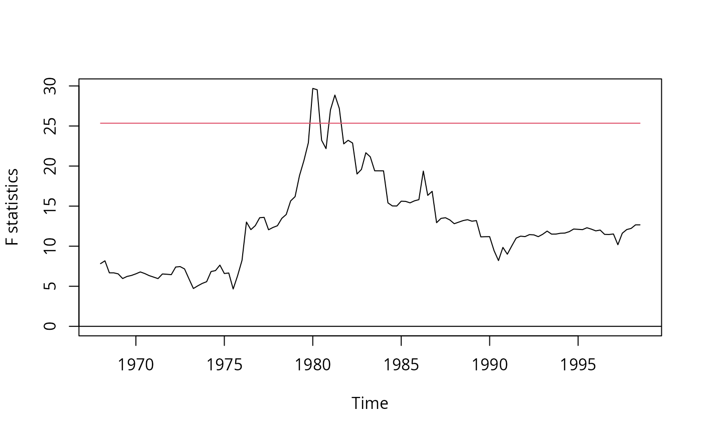 ## alternatively: re-use fm_adl44
mf <- model.frame(fm_adl44)
mf <- ts(as.matrix(mf), start = c(1962, 1), freq = 4)
colnames(mf) <- c("y", paste("x", 1:8, sep = ""))
ff <- as.formula(paste("y", "~", paste("x", 1:8, sep = "", collapse = " + ")))
fs <- Fstats(ff, data = mf, from = 0.1)
plot(fs)
lines(boundary(fs, alpha = 0.01), lty = 2, col = 2)
lines(boundary(fs, alpha = 0.1), lty = 3, col = 2)
## alternatively: re-use fm_adl44
mf <- model.frame(fm_adl44)
mf <- ts(as.matrix(mf), start = c(1962, 1), freq = 4)
colnames(mf) <- c("y", paste("x", 1:8, sep = ""))
ff <- as.formula(paste("y", "~", paste("x", 1:8, sep = "", collapse = " + ")))
fs <- Fstats(ff, data = mf, from = 0.1)
plot(fs)
lines(boundary(fs, alpha = 0.01), lty = 2, col = 2)
lines(boundary(fs, alpha = 0.1), lty = 3, col = 2)
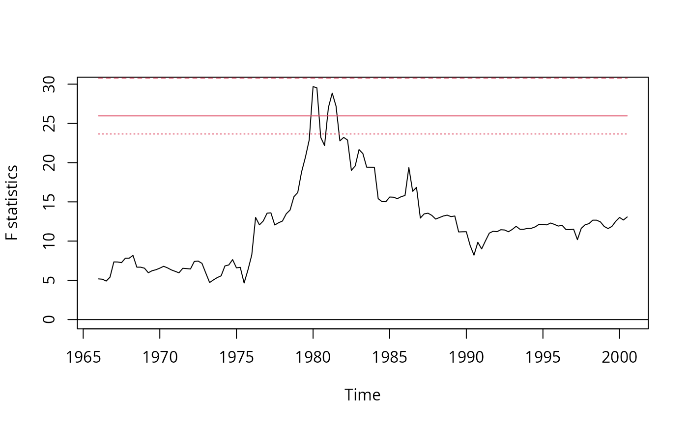 ##########################################
## Monthly US stock returns (1931-2002) ##
##########################################
## package and data
library("dynlm")
data("USStocksSW", package = "AER")
## Table 14.3, p. 540
fm1 <- dynlm(returns ~ L(returns), data = USStocksSW, start = c(1960,1))
coeftest(fm1, vcov = sandwich)
#>
#> t test of coefficients:
#>
#> Estimate Std. Error t value Pr(>|t|)
#> (Intercept) 0.311562 0.197371 1.5786 0.1151
#> L(returns) 0.050390 0.051208 0.9840 0.3256
#>
fm2 <- dynlm(returns ~ L(returns, 1:2), data = USStocksSW, start = c(1960,1))
waldtest(fm2, vcov = sandwich)
#> Wald test
#>
#> Model 1: returns ~ L(returns, 1:2)
#> Model 2: returns ~ 1
#> Res.Df Df F Pr(>F)
#> 1 513
#> 2 515 -2 1.3423 0.2622
fm3 <- dynlm(returns ~ L(returns, 1:4), data = USStocksSW, start = c(1960,1))
waldtest(fm3, vcov = sandwich)
#> Wald test
#>
#> Model 1: returns ~ L(returns, 1:4)
#> Model 2: returns ~ 1
#> Res.Df Df F Pr(>F)
#> 1 511
#> 2 515 -4 0.7069 0.5875
## Table 14.7, p. 574
fm4 <- dynlm(returns ~ L(returns) + L(d(dividend)),
data = USStocksSW, start = c(1960, 1))
fm5 <- dynlm(returns ~ L(returns, 1:2) + L(d(dividend), 1:2),
data = USStocksSW, start = c(1960, 1))
fm6 <- dynlm(returns ~ L(returns) + L(dividend),
data = USStocksSW, start = c(1960, 1))
##################################
## Price of frozen orange juice ##
##################################
## load data
data("FrozenJuice")
## Stock and Watson, p. 594
library("dynlm")
fm_dyn <- dynlm(d(100 * log(price/ppi)) ~ fdd, data = FrozenJuice)
coeftest(fm_dyn, vcov = vcovHC(fm_dyn, type = "HC1"))
#>
#> t test of coefficients:
#>
#> Estimate Std. Error t value Pr(>|t|)
#> (Intercept) -0.42095 0.18877 -2.2299 0.0261146 *
#> fdd 0.46724 0.13390 3.4894 0.0005191 ***
#> ---
#> Signif. codes: 0 ‘***’ 0.001 ‘**’ 0.01 ‘*’ 0.05 ‘.’ 0.1 ‘ ’ 1
#>
## equivalently, returns can be computed 'by hand'
## (reducing the complexity of the formula notation)
fj <- ts.union(fdd = FrozenJuice[, "fdd"],
ret = 100 * diff(log(FrozenJuice[,"price"]/FrozenJuice[,"ppi"])))
fm_dyn <- dynlm(ret ~ fdd, data = fj)
## Stock and Watson, p. 595
fm_dl <- dynlm(ret ~ L(fdd, 0:6), data = fj)
coeftest(fm_dl, vcov = vcovHC(fm_dl, type = "HC1"))
#>
#> t test of coefficients:
#>
#> Estimate Std. Error t value Pr(>|t|)
#> (Intercept) -0.692961 0.209677 -3.3049 0.0010069 **
#> L(fdd, 0:6)0 0.471433 0.135041 3.4910 0.0005166 ***
#> L(fdd, 0:6)1 0.145021 0.081243 1.7850 0.0747619 .
#> L(fdd, 0:6)2 0.058364 0.059050 0.9884 0.3233652
#> L(fdd, 0:6)3 0.074166 0.047230 1.5703 0.1168744
#> L(fdd, 0:6)4 0.036304 0.029296 1.2392 0.2157537
#> L(fdd, 0:6)5 0.048756 0.031369 1.5543 0.1206451
#> L(fdd, 0:6)6 0.050246 0.045053 1.1153 0.2651845
#> ---
#> Signif. codes: 0 ‘***’ 0.001 ‘**’ 0.01 ‘*’ 0.05 ‘.’ 0.1 ‘ ’ 1
#>
## Stock and Watson, Table 15.1, p. 620, numbers refer to columns
## (1) Dynamic Multipliers
fm1 <- dynlm(ret ~ L(fdd, 0:18), data = fj)
coeftest(fm1, vcov = NeweyWest(fm1, lag = 7, prewhite = FALSE))
#>
#> t test of coefficients:
#>
#> Estimate Std. Error t value Pr(>|t|)
#> (Intercept) -0.3433429 0.2690139 -1.2763 0.2023649
#> L(fdd, 0:18)0 0.5076608 0.1374819 3.6926 0.0002432 ***
#> L(fdd, 0:18)1 0.1724593 0.0877213 1.9660 0.0497811 *
#> L(fdd, 0:18)2 0.0682814 0.0598434 1.1410 0.2543456
#> L(fdd, 0:18)3 0.0702622 0.0441531 1.5913 0.1120856
#> L(fdd, 0:18)4 0.0224493 0.0313514 0.7161 0.4742498
#> L(fdd, 0:18)5 0.0270402 0.0298585 0.9056 0.3655222
#> L(fdd, 0:18)6 0.0313550 0.0470457 0.6665 0.5053724
#> L(fdd, 0:18)7 0.0150871 0.0153622 0.9821 0.3264662
#> L(fdd, 0:18)8 -0.0420438 0.0343135 -1.2253 0.2209703
#> L(fdd, 0:18)9 -0.0101323 0.0506565 -0.2000 0.8415365
#> L(fdd, 0:18)10 -0.1161595 0.0694595 -1.6723 0.0950032 .
#> L(fdd, 0:18)11 -0.0666059 0.0522360 -1.2751 0.2027914
#> L(fdd, 0:18)12 -0.1430786 0.0760642 -1.8810 0.0604743 .
#> L(fdd, 0:18)13 -0.0827249 0.0425512 -1.9441 0.0523683 .
#> L(fdd, 0:18)14 -0.0567700 0.0348143 -1.6307 0.1035125
#> L(fdd, 0:18)15 -0.0315207 0.0275916 -1.1424 0.2537643
#> L(fdd, 0:18)16 -0.0054563 0.0548472 -0.0995 0.9207910
#> L(fdd, 0:18)17 0.0029145 0.0182780 0.1595 0.8733689
#> L(fdd, 0:18)18 0.0030657 0.0167679 0.1828 0.8549946
#> ---
#> Signif. codes: 0 ‘***’ 0.001 ‘**’ 0.01 ‘*’ 0.05 ‘.’ 0.1 ‘ ’ 1
#>
## (2) Cumulative Multipliers
fm2 <- dynlm(ret ~ L(d(fdd), 0:17) + L(fdd, 18), data = fj)
coeftest(fm2, vcov = NeweyWest(fm2, lag = 7, prewhite = FALSE))
#>
#> t test of coefficients:
#>
#> Estimate Std. Error t value Pr(>|t|)
#> (Intercept) -0.34334 0.26901 -1.2763 0.2023649
#> L(d(fdd), 0:17)0 0.50766 0.13748 3.6926 0.0002432 ***
#> L(d(fdd), 0:17)1 0.68012 0.13371 5.0867 4.943e-07 ***
#> L(d(fdd), 0:17)2 0.74840 0.16506 4.5342 7.043e-06 ***
#> L(d(fdd), 0:17)3 0.81866 0.18122 4.5176 7.598e-06 ***
#> L(d(fdd), 0:17)4 0.84111 0.18262 4.6059 5.063e-06 ***
#> L(d(fdd), 0:17)5 0.86815 0.18929 4.5863 5.543e-06 ***
#> L(d(fdd), 0:17)6 0.89951 0.20167 4.4603 9.851e-06 ***
#> L(d(fdd), 0:17)7 0.91460 0.20484 4.4648 9.651e-06 ***
#> L(d(fdd), 0:17)8 0.87255 0.21388 4.0797 5.148e-05 ***
#> L(d(fdd), 0:17)9 0.86242 0.23592 3.6555 0.0002802 ***
#> L(d(fdd), 0:17)10 0.74626 0.25685 2.9054 0.0038090 **
#> L(d(fdd), 0:17)11 0.67965 0.26602 2.5549 0.0108797 *
#> L(d(fdd), 0:17)12 0.53658 0.26788 2.0030 0.0456462 *
#> L(d(fdd), 0:17)13 0.45385 0.26741 1.6972 0.0902037 .
#> L(d(fdd), 0:17)14 0.39708 0.27347 1.4520 0.1470508
#> L(d(fdd), 0:17)15 0.36556 0.27579 1.3255 0.1855343
#> L(d(fdd), 0:17)16 0.36010 0.28322 1.2714 0.2040869
#> L(d(fdd), 0:17)17 0.36302 0.28661 1.2666 0.2058109
#> L(fdd, 18) 0.36608 0.29298 1.2495 0.2119777
#> ---
#> Signif. codes: 0 ‘***’ 0.001 ‘**’ 0.01 ‘*’ 0.05 ‘.’ 0.1 ‘ ’ 1
#>
## (3) Cumulative Multipliers, more lags in NW
coeftest(fm2, vcov = NeweyWest(fm2, lag = 14, prewhite = FALSE))
#>
#> t test of coefficients:
#>
#> Estimate Std. Error t value Pr(>|t|)
#> (Intercept) -0.34334 0.25590 -1.3417 0.1802166
#> L(d(fdd), 0:17)0 0.50766 0.13920 3.6469 0.0002896 ***
#> L(d(fdd), 0:17)1 0.68012 0.12984 5.2381 2.281e-07 ***
#> L(d(fdd), 0:17)2 0.74840 0.16243 4.6076 5.024e-06 ***
#> L(d(fdd), 0:17)3 0.81866 0.18129 4.5158 7.659e-06 ***
#> L(d(fdd), 0:17)4 0.84111 0.18389 4.5740 5.866e-06 ***
#> L(d(fdd), 0:17)5 0.86815 0.18902 4.5930 5.375e-06 ***
#> L(d(fdd), 0:17)6 0.89951 0.20787 4.3273 1.781e-05 ***
#> L(d(fdd), 0:17)7 0.91460 0.20958 4.3640 1.515e-05 ***
#> L(d(fdd), 0:17)8 0.87255 0.21849 3.9935 7.356e-05 ***
#> L(d(fdd), 0:17)9 0.86242 0.24462 3.5255 0.0004564 ***
#> L(d(fdd), 0:17)10 0.74626 0.26198 2.8485 0.0045497 **
#> L(d(fdd), 0:17)11 0.67965 0.27166 2.5018 0.0126321 *
#> L(d(fdd), 0:17)12 0.53658 0.27089 1.9808 0.0480945 *
#> L(d(fdd), 0:17)13 0.45385 0.27250 1.6655 0.0963629 .
#> L(d(fdd), 0:17)14 0.39708 0.28431 1.3966 0.1630649
#> L(d(fdd), 0:17)15 0.36556 0.28662 1.2754 0.2026772
#> L(d(fdd), 0:17)16 0.36010 0.29306 1.2288 0.2196603
#> L(d(fdd), 0:17)17 0.36302 0.29402 1.2347 0.2174650
#> L(fdd, 18) 0.36608 0.30064 1.2177 0.2238504
#> ---
#> Signif. codes: 0 ‘***’ 0.001 ‘**’ 0.01 ‘*’ 0.05 ‘.’ 0.1 ‘ ’ 1
#>
## (4) Cumulative Multipliers with monthly indicators
fm4 <- dynlm(ret ~ L(d(fdd), 0:17) + L(fdd, 18) + season(fdd), data = fj)
coeftest(fm4, vcov = NeweyWest(fm4, lag = 7, prewhite = FALSE))
#>
#> t test of coefficients:
#>
#> Estimate Std. Error t value Pr(>|t|)
#> (Intercept) -0.24056 0.93399 -0.2576 0.7968380
#> L(d(fdd), 0:17)0 0.52362 0.14188 3.6906 0.0002455 ***
#> L(d(fdd), 0:17)1 0.72019 0.14237 5.0587 5.722e-07 ***
#> L(d(fdd), 0:17)2 0.78083 0.17335 4.5044 8.095e-06 ***
#> L(d(fdd), 0:17)3 0.86075 0.18956 4.5407 6.861e-06 ***
#> L(d(fdd), 0:17)4 0.89180 0.19403 4.5962 5.315e-06 ***
#> L(d(fdd), 0:17)5 0.90445 0.19935 4.5369 6.980e-06 ***
#> L(d(fdd), 0:17)6 0.92233 0.21031 4.3857 1.380e-05 ***
#> L(d(fdd), 0:17)7 0.93899 0.21200 4.4292 1.137e-05 ***
#> L(d(fdd), 0:17)8 0.90441 0.21873 4.1348 4.094e-05 ***
#> L(d(fdd), 0:17)9 0.88400 0.23857 3.7054 0.0002319 ***
#> L(d(fdd), 0:17)10 0.75191 0.25890 2.9042 0.0038258 **
#> L(d(fdd), 0:17)11 0.67739 0.26680 2.5390 0.0113855 *
#> L(d(fdd), 0:17)12 0.55126 0.27219 2.0253 0.0433104 *
#> L(d(fdd), 0:17)13 0.49131 0.27496 1.7869 0.0744964 .
#> L(d(fdd), 0:17)14 0.42678 0.27777 1.5364 0.1249936
#> L(d(fdd), 0:17)15 0.40648 0.28003 1.4515 0.1471914
#> L(d(fdd), 0:17)16 0.40784 0.28647 1.4237 0.1550965
#> L(d(fdd), 0:17)17 0.39548 0.29007 1.3634 0.1732990
#> L(fdd, 18) 0.38589 0.29481 1.3089 0.1910934
#> season(fdd)Feb -0.95658 1.56798 -0.6101 0.5420614
#> season(fdd)Mar -0.63580 1.02093 -0.6228 0.5336885
#> season(fdd)Apr 0.50068 1.06515 0.4701 0.6385002
#> season(fdd)May -1.08018 1.50233 -0.7190 0.4724398
#> season(fdd)Jun 0.31956 1.12814 0.2833 0.7770784
#> season(fdd)Jul 0.19511 1.11215 0.1754 0.8607997
#> season(fdd)Aug 0.36443 1.01074 0.3606 0.7185657
#> season(fdd)Sep -0.41310 0.98887 -0.4177 0.6762921
#> season(fdd)Oct -0.15666 0.93696 -0.1672 0.8672709
#> season(fdd)Nov 0.31165 1.12787 0.2763 0.7824033
#> season(fdd)Dec 0.14816 1.26534 0.1171 0.9068306
#> ---
#> Signif. codes: 0 ‘***’ 0.001 ‘**’ 0.01 ‘*’ 0.05 ‘.’ 0.1 ‘ ’ 1
#>
## monthly indicators needed?
fm4r <- update(fm4, . ~ . - season(fdd))
waldtest(fm4, fm4r, vcov= NeweyWest(fm4, lag = 7, prewhite = FALSE)) ## close ...
#> Wald test
#>
#> Model 1: ret ~ L(d(fdd), 0:17) + L(fdd, 18) + season(fdd)
#> Model 2: ret ~ L(d(fdd), 0:17) + L(fdd, 18)
#> Res.Df Df F Pr(>F)
#> 1 563
#> 2 574 -11 0.9683 0.4743
#############################################
## New York Stock Exchange composite index ##
#############################################
## returns
data("NYSESW", package = "AER")
ret <- 100 * diff(log(NYSESW))
plot(ret)
##########################################
## Monthly US stock returns (1931-2002) ##
##########################################
## package and data
library("dynlm")
data("USStocksSW", package = "AER")
## Table 14.3, p. 540
fm1 <- dynlm(returns ~ L(returns), data = USStocksSW, start = c(1960,1))
coeftest(fm1, vcov = sandwich)
#>
#> t test of coefficients:
#>
#> Estimate Std. Error t value Pr(>|t|)
#> (Intercept) 0.311562 0.197371 1.5786 0.1151
#> L(returns) 0.050390 0.051208 0.9840 0.3256
#>
fm2 <- dynlm(returns ~ L(returns, 1:2), data = USStocksSW, start = c(1960,1))
waldtest(fm2, vcov = sandwich)
#> Wald test
#>
#> Model 1: returns ~ L(returns, 1:2)
#> Model 2: returns ~ 1
#> Res.Df Df F Pr(>F)
#> 1 513
#> 2 515 -2 1.3423 0.2622
fm3 <- dynlm(returns ~ L(returns, 1:4), data = USStocksSW, start = c(1960,1))
waldtest(fm3, vcov = sandwich)
#> Wald test
#>
#> Model 1: returns ~ L(returns, 1:4)
#> Model 2: returns ~ 1
#> Res.Df Df F Pr(>F)
#> 1 511
#> 2 515 -4 0.7069 0.5875
## Table 14.7, p. 574
fm4 <- dynlm(returns ~ L(returns) + L(d(dividend)),
data = USStocksSW, start = c(1960, 1))
fm5 <- dynlm(returns ~ L(returns, 1:2) + L(d(dividend), 1:2),
data = USStocksSW, start = c(1960, 1))
fm6 <- dynlm(returns ~ L(returns) + L(dividend),
data = USStocksSW, start = c(1960, 1))
##################################
## Price of frozen orange juice ##
##################################
## load data
data("FrozenJuice")
## Stock and Watson, p. 594
library("dynlm")
fm_dyn <- dynlm(d(100 * log(price/ppi)) ~ fdd, data = FrozenJuice)
coeftest(fm_dyn, vcov = vcovHC(fm_dyn, type = "HC1"))
#>
#> t test of coefficients:
#>
#> Estimate Std. Error t value Pr(>|t|)
#> (Intercept) -0.42095 0.18877 -2.2299 0.0261146 *
#> fdd 0.46724 0.13390 3.4894 0.0005191 ***
#> ---
#> Signif. codes: 0 ‘***’ 0.001 ‘**’ 0.01 ‘*’ 0.05 ‘.’ 0.1 ‘ ’ 1
#>
## equivalently, returns can be computed 'by hand'
## (reducing the complexity of the formula notation)
fj <- ts.union(fdd = FrozenJuice[, "fdd"],
ret = 100 * diff(log(FrozenJuice[,"price"]/FrozenJuice[,"ppi"])))
fm_dyn <- dynlm(ret ~ fdd, data = fj)
## Stock and Watson, p. 595
fm_dl <- dynlm(ret ~ L(fdd, 0:6), data = fj)
coeftest(fm_dl, vcov = vcovHC(fm_dl, type = "HC1"))
#>
#> t test of coefficients:
#>
#> Estimate Std. Error t value Pr(>|t|)
#> (Intercept) -0.692961 0.209677 -3.3049 0.0010069 **
#> L(fdd, 0:6)0 0.471433 0.135041 3.4910 0.0005166 ***
#> L(fdd, 0:6)1 0.145021 0.081243 1.7850 0.0747619 .
#> L(fdd, 0:6)2 0.058364 0.059050 0.9884 0.3233652
#> L(fdd, 0:6)3 0.074166 0.047230 1.5703 0.1168744
#> L(fdd, 0:6)4 0.036304 0.029296 1.2392 0.2157537
#> L(fdd, 0:6)5 0.048756 0.031369 1.5543 0.1206451
#> L(fdd, 0:6)6 0.050246 0.045053 1.1153 0.2651845
#> ---
#> Signif. codes: 0 ‘***’ 0.001 ‘**’ 0.01 ‘*’ 0.05 ‘.’ 0.1 ‘ ’ 1
#>
## Stock and Watson, Table 15.1, p. 620, numbers refer to columns
## (1) Dynamic Multipliers
fm1 <- dynlm(ret ~ L(fdd, 0:18), data = fj)
coeftest(fm1, vcov = NeweyWest(fm1, lag = 7, prewhite = FALSE))
#>
#> t test of coefficients:
#>
#> Estimate Std. Error t value Pr(>|t|)
#> (Intercept) -0.3433429 0.2690139 -1.2763 0.2023649
#> L(fdd, 0:18)0 0.5076608 0.1374819 3.6926 0.0002432 ***
#> L(fdd, 0:18)1 0.1724593 0.0877213 1.9660 0.0497811 *
#> L(fdd, 0:18)2 0.0682814 0.0598434 1.1410 0.2543456
#> L(fdd, 0:18)3 0.0702622 0.0441531 1.5913 0.1120856
#> L(fdd, 0:18)4 0.0224493 0.0313514 0.7161 0.4742498
#> L(fdd, 0:18)5 0.0270402 0.0298585 0.9056 0.3655222
#> L(fdd, 0:18)6 0.0313550 0.0470457 0.6665 0.5053724
#> L(fdd, 0:18)7 0.0150871 0.0153622 0.9821 0.3264662
#> L(fdd, 0:18)8 -0.0420438 0.0343135 -1.2253 0.2209703
#> L(fdd, 0:18)9 -0.0101323 0.0506565 -0.2000 0.8415365
#> L(fdd, 0:18)10 -0.1161595 0.0694595 -1.6723 0.0950032 .
#> L(fdd, 0:18)11 -0.0666059 0.0522360 -1.2751 0.2027914
#> L(fdd, 0:18)12 -0.1430786 0.0760642 -1.8810 0.0604743 .
#> L(fdd, 0:18)13 -0.0827249 0.0425512 -1.9441 0.0523683 .
#> L(fdd, 0:18)14 -0.0567700 0.0348143 -1.6307 0.1035125
#> L(fdd, 0:18)15 -0.0315207 0.0275916 -1.1424 0.2537643
#> L(fdd, 0:18)16 -0.0054563 0.0548472 -0.0995 0.9207910
#> L(fdd, 0:18)17 0.0029145 0.0182780 0.1595 0.8733689
#> L(fdd, 0:18)18 0.0030657 0.0167679 0.1828 0.8549946
#> ---
#> Signif. codes: 0 ‘***’ 0.001 ‘**’ 0.01 ‘*’ 0.05 ‘.’ 0.1 ‘ ’ 1
#>
## (2) Cumulative Multipliers
fm2 <- dynlm(ret ~ L(d(fdd), 0:17) + L(fdd, 18), data = fj)
coeftest(fm2, vcov = NeweyWest(fm2, lag = 7, prewhite = FALSE))
#>
#> t test of coefficients:
#>
#> Estimate Std. Error t value Pr(>|t|)
#> (Intercept) -0.34334 0.26901 -1.2763 0.2023649
#> L(d(fdd), 0:17)0 0.50766 0.13748 3.6926 0.0002432 ***
#> L(d(fdd), 0:17)1 0.68012 0.13371 5.0867 4.943e-07 ***
#> L(d(fdd), 0:17)2 0.74840 0.16506 4.5342 7.043e-06 ***
#> L(d(fdd), 0:17)3 0.81866 0.18122 4.5176 7.598e-06 ***
#> L(d(fdd), 0:17)4 0.84111 0.18262 4.6059 5.063e-06 ***
#> L(d(fdd), 0:17)5 0.86815 0.18929 4.5863 5.543e-06 ***
#> L(d(fdd), 0:17)6 0.89951 0.20167 4.4603 9.851e-06 ***
#> L(d(fdd), 0:17)7 0.91460 0.20484 4.4648 9.651e-06 ***
#> L(d(fdd), 0:17)8 0.87255 0.21388 4.0797 5.148e-05 ***
#> L(d(fdd), 0:17)9 0.86242 0.23592 3.6555 0.0002802 ***
#> L(d(fdd), 0:17)10 0.74626 0.25685 2.9054 0.0038090 **
#> L(d(fdd), 0:17)11 0.67965 0.26602 2.5549 0.0108797 *
#> L(d(fdd), 0:17)12 0.53658 0.26788 2.0030 0.0456462 *
#> L(d(fdd), 0:17)13 0.45385 0.26741 1.6972 0.0902037 .
#> L(d(fdd), 0:17)14 0.39708 0.27347 1.4520 0.1470508
#> L(d(fdd), 0:17)15 0.36556 0.27579 1.3255 0.1855343
#> L(d(fdd), 0:17)16 0.36010 0.28322 1.2714 0.2040869
#> L(d(fdd), 0:17)17 0.36302 0.28661 1.2666 0.2058109
#> L(fdd, 18) 0.36608 0.29298 1.2495 0.2119777
#> ---
#> Signif. codes: 0 ‘***’ 0.001 ‘**’ 0.01 ‘*’ 0.05 ‘.’ 0.1 ‘ ’ 1
#>
## (3) Cumulative Multipliers, more lags in NW
coeftest(fm2, vcov = NeweyWest(fm2, lag = 14, prewhite = FALSE))
#>
#> t test of coefficients:
#>
#> Estimate Std. Error t value Pr(>|t|)
#> (Intercept) -0.34334 0.25590 -1.3417 0.1802166
#> L(d(fdd), 0:17)0 0.50766 0.13920 3.6469 0.0002896 ***
#> L(d(fdd), 0:17)1 0.68012 0.12984 5.2381 2.281e-07 ***
#> L(d(fdd), 0:17)2 0.74840 0.16243 4.6076 5.024e-06 ***
#> L(d(fdd), 0:17)3 0.81866 0.18129 4.5158 7.659e-06 ***
#> L(d(fdd), 0:17)4 0.84111 0.18389 4.5740 5.866e-06 ***
#> L(d(fdd), 0:17)5 0.86815 0.18902 4.5930 5.375e-06 ***
#> L(d(fdd), 0:17)6 0.89951 0.20787 4.3273 1.781e-05 ***
#> L(d(fdd), 0:17)7 0.91460 0.20958 4.3640 1.515e-05 ***
#> L(d(fdd), 0:17)8 0.87255 0.21849 3.9935 7.356e-05 ***
#> L(d(fdd), 0:17)9 0.86242 0.24462 3.5255 0.0004564 ***
#> L(d(fdd), 0:17)10 0.74626 0.26198 2.8485 0.0045497 **
#> L(d(fdd), 0:17)11 0.67965 0.27166 2.5018 0.0126321 *
#> L(d(fdd), 0:17)12 0.53658 0.27089 1.9808 0.0480945 *
#> L(d(fdd), 0:17)13 0.45385 0.27250 1.6655 0.0963629 .
#> L(d(fdd), 0:17)14 0.39708 0.28431 1.3966 0.1630649
#> L(d(fdd), 0:17)15 0.36556 0.28662 1.2754 0.2026772
#> L(d(fdd), 0:17)16 0.36010 0.29306 1.2288 0.2196603
#> L(d(fdd), 0:17)17 0.36302 0.29402 1.2347 0.2174650
#> L(fdd, 18) 0.36608 0.30064 1.2177 0.2238504
#> ---
#> Signif. codes: 0 ‘***’ 0.001 ‘**’ 0.01 ‘*’ 0.05 ‘.’ 0.1 ‘ ’ 1
#>
## (4) Cumulative Multipliers with monthly indicators
fm4 <- dynlm(ret ~ L(d(fdd), 0:17) + L(fdd, 18) + season(fdd), data = fj)
coeftest(fm4, vcov = NeweyWest(fm4, lag = 7, prewhite = FALSE))
#>
#> t test of coefficients:
#>
#> Estimate Std. Error t value Pr(>|t|)
#> (Intercept) -0.24056 0.93399 -0.2576 0.7968380
#> L(d(fdd), 0:17)0 0.52362 0.14188 3.6906 0.0002455 ***
#> L(d(fdd), 0:17)1 0.72019 0.14237 5.0587 5.722e-07 ***
#> L(d(fdd), 0:17)2 0.78083 0.17335 4.5044 8.095e-06 ***
#> L(d(fdd), 0:17)3 0.86075 0.18956 4.5407 6.861e-06 ***
#> L(d(fdd), 0:17)4 0.89180 0.19403 4.5962 5.315e-06 ***
#> L(d(fdd), 0:17)5 0.90445 0.19935 4.5369 6.980e-06 ***
#> L(d(fdd), 0:17)6 0.92233 0.21031 4.3857 1.380e-05 ***
#> L(d(fdd), 0:17)7 0.93899 0.21200 4.4292 1.137e-05 ***
#> L(d(fdd), 0:17)8 0.90441 0.21873 4.1348 4.094e-05 ***
#> L(d(fdd), 0:17)9 0.88400 0.23857 3.7054 0.0002319 ***
#> L(d(fdd), 0:17)10 0.75191 0.25890 2.9042 0.0038258 **
#> L(d(fdd), 0:17)11 0.67739 0.26680 2.5390 0.0113855 *
#> L(d(fdd), 0:17)12 0.55126 0.27219 2.0253 0.0433104 *
#> L(d(fdd), 0:17)13 0.49131 0.27496 1.7869 0.0744964 .
#> L(d(fdd), 0:17)14 0.42678 0.27777 1.5364 0.1249936
#> L(d(fdd), 0:17)15 0.40648 0.28003 1.4515 0.1471914
#> L(d(fdd), 0:17)16 0.40784 0.28647 1.4237 0.1550965
#> L(d(fdd), 0:17)17 0.39548 0.29007 1.3634 0.1732990
#> L(fdd, 18) 0.38589 0.29481 1.3089 0.1910934
#> season(fdd)Feb -0.95658 1.56798 -0.6101 0.5420614
#> season(fdd)Mar -0.63580 1.02093 -0.6228 0.5336885
#> season(fdd)Apr 0.50068 1.06515 0.4701 0.6385002
#> season(fdd)May -1.08018 1.50233 -0.7190 0.4724398
#> season(fdd)Jun 0.31956 1.12814 0.2833 0.7770784
#> season(fdd)Jul 0.19511 1.11215 0.1754 0.8607997
#> season(fdd)Aug 0.36443 1.01074 0.3606 0.7185657
#> season(fdd)Sep -0.41310 0.98887 -0.4177 0.6762921
#> season(fdd)Oct -0.15666 0.93696 -0.1672 0.8672709
#> season(fdd)Nov 0.31165 1.12787 0.2763 0.7824033
#> season(fdd)Dec 0.14816 1.26534 0.1171 0.9068306
#> ---
#> Signif. codes: 0 ‘***’ 0.001 ‘**’ 0.01 ‘*’ 0.05 ‘.’ 0.1 ‘ ’ 1
#>
## monthly indicators needed?
fm4r <- update(fm4, . ~ . - season(fdd))
waldtest(fm4, fm4r, vcov= NeweyWest(fm4, lag = 7, prewhite = FALSE)) ## close ...
#> Wald test
#>
#> Model 1: ret ~ L(d(fdd), 0:17) + L(fdd, 18) + season(fdd)
#> Model 2: ret ~ L(d(fdd), 0:17) + L(fdd, 18)
#> Res.Df Df F Pr(>F)
#> 1 563
#> 2 574 -11 0.9683 0.4743
#############################################
## New York Stock Exchange composite index ##
#############################################
## returns
data("NYSESW", package = "AER")
ret <- 100 * diff(log(NYSESW))
plot(ret)
 ## fit GARCH(1,1)
library("tseries")
fm <- garch(coredata(ret))
#>
#> ***** ESTIMATION WITH ANALYTICAL GRADIENT *****
#>
#>
#> I INITIAL X(I) D(I)
#>
#> 1 7.247660e-01 1.000e+00
#> 2 5.000000e-02 1.000e+00
#> 3 5.000000e-02 1.000e+00
#>
#> IT NF F RELDF PRELDF RELDX STPPAR D*STEP NPRELDF
#> 0 1 1.503e+03
#> 1 3 1.487e+03 1.08e-02 2.29e-01 3.2e-01 1.7e+03 4.5e-01 1.96e+02
#> 2 4 1.481e+03 3.49e-03 6.05e-02 1.8e-01 2.7e+00 2.2e-01 6.80e+01
#> 3 5 1.406e+03 5.06e-02 6.85e-02 1.1e-01 2.3e+00 1.1e-01 8.55e+01
#> 4 7 1.374e+03 2.31e-02 2.63e-02 9.2e-02 1.2e+01 1.1e-01 6.91e+01
#> 5 9 1.356e+03 1.30e-02 2.07e-02 1.2e-01 4.0e+00 1.0e-01 1.06e+01
#> 6 10 1.330e+03 1.91e-02 2.08e-02 1.4e-01 2.0e+00 1.0e-01 1.47e+01
#> 7 11 1.297e+03 2.52e-02 3.20e-02 1.7e-01 2.0e+00 2.0e-01 1.11e+01
#> 8 13 1.290e+03 5.19e-03 1.02e-02 3.4e-02 2.9e+00 4.0e-02 1.85e+00
#> 9 14 1.278e+03 9.38e-03 1.03e-02 2.9e-02 2.0e+00 4.0e-02 2.39e+00
#> 10 15 1.261e+03 1.29e-02 1.58e-02 7.6e-02 2.0e+00 8.0e-02 1.92e+00
#> 11 16 1.227e+03 2.73e-02 3.26e-02 1.2e-01 2.0e+00 1.6e-01 2.11e+00
#> 12 18 1.223e+03 3.24e-03 9.12e-03 1.3e-02 1.8e+02 2.5e-02 4.47e+00
#> 13 19 1.212e+03 9.29e-03 9.02e-03 1.4e-02 2.0e+00 2.5e-02 1.59e+00
#> 14 22 1.168e+03 3.63e-02 3.40e-02 7.2e-02 1.8e+00 1.3e-01 1.70e+00
#> 15 24 1.162e+03 4.48e-03 7.20e-03 1.5e-02 2.0e+00 2.6e-02 5.64e+00
#> 16 25 1.150e+03 1.06e-02 1.12e-02 1.5e-02 2.0e+00 2.6e-02 3.37e+00
#> 17 27 1.135e+03 1.34e-02 1.43e-02 2.4e-02 2.0e+00 5.3e-02 3.34e+00
#> 18 28 1.118e+03 1.50e-02 3.01e-02 4.8e-02 1.9e+00 1.1e-01 9.31e-01
#> 19 31 1.111e+03 5.86e-03 8.61e-03 1.3e-03 4.0e+00 3.4e-03 9.54e-01
#> 20 33 1.102e+03 7.77e-03 1.33e-02 5.4e-03 1.6e+01 1.3e-02 1.18e+00
#> 21 37 1.102e+03 5.75e-04 9.10e-04 5.0e-04 3.8e+00 1.2e-03 3.59e-01
#> 22 39 1.101e+03 4.98e-04 5.37e-04 1.6e-03 2.1e+00 3.4e-03 2.75e-01
#> 23 40 1.100e+03 1.37e-03 1.55e-03 2.9e-03 2.0e+00 6.7e-03 2.23e-01
#> 24 43 1.096e+03 3.56e-03 6.62e-03 1.6e-02 1.8e+00 3.9e-02 9.44e-02
#> 25 45 1.095e+03 6.89e-04 8.79e-04 3.2e-03 1.0e+00 7.0e-03 1.17e-03
#> 26 47 1.095e+03 1.16e-04 1.90e-04 4.8e-04 1.0e+00 1.2e-03 3.08e-04
#> 27 48 1.095e+03 7.85e-07 9.55e-07 1.2e-04 0.0e+00 2.9e-04 9.55e-07
#> 28 49 1.095e+03 3.91e-08 9.27e-08 5.4e-05 0.0e+00 1.2e-04 9.27e-08
#> 29 50 1.095e+03 3.73e-09 1.07e-09 8.4e-06 0.0e+00 2.1e-05 1.07e-09
#> 30 51 1.095e+03 -1.54e-10 8.11e-11 1.6e-06 0.0e+00 4.0e-06 8.11e-11
#>
#> ***** RELATIVE FUNCTION CONVERGENCE *****
#>
#> FUNCTION 1.094921e+03 RELDX 1.590e-06
#> FUNC. EVALS 51 GRAD. EVALS 30
#> PRELDF 8.114e-11 NPRELDF 8.114e-11
#>
#> I FINAL X(I) D(I) G(I)
#>
#> 1 7.620546e-03 1.000e+00 3.522e-01
#> 2 7.019513e-02 1.000e+00 8.588e-02
#> 3 9.216098e-01 1.000e+00 1.571e-01
#>
## fit GARCH(1,1)
library("tseries")
fm <- garch(coredata(ret))
#>
#> ***** ESTIMATION WITH ANALYTICAL GRADIENT *****
#>
#>
#> I INITIAL X(I) D(I)
#>
#> 1 7.247660e-01 1.000e+00
#> 2 5.000000e-02 1.000e+00
#> 3 5.000000e-02 1.000e+00
#>
#> IT NF F RELDF PRELDF RELDX STPPAR D*STEP NPRELDF
#> 0 1 1.503e+03
#> 1 3 1.487e+03 1.08e-02 2.29e-01 3.2e-01 1.7e+03 4.5e-01 1.96e+02
#> 2 4 1.481e+03 3.49e-03 6.05e-02 1.8e-01 2.7e+00 2.2e-01 6.80e+01
#> 3 5 1.406e+03 5.06e-02 6.85e-02 1.1e-01 2.3e+00 1.1e-01 8.55e+01
#> 4 7 1.374e+03 2.31e-02 2.63e-02 9.2e-02 1.2e+01 1.1e-01 6.91e+01
#> 5 9 1.356e+03 1.30e-02 2.07e-02 1.2e-01 4.0e+00 1.0e-01 1.06e+01
#> 6 10 1.330e+03 1.91e-02 2.08e-02 1.4e-01 2.0e+00 1.0e-01 1.47e+01
#> 7 11 1.297e+03 2.52e-02 3.20e-02 1.7e-01 2.0e+00 2.0e-01 1.11e+01
#> 8 13 1.290e+03 5.19e-03 1.02e-02 3.4e-02 2.9e+00 4.0e-02 1.85e+00
#> 9 14 1.278e+03 9.38e-03 1.03e-02 2.9e-02 2.0e+00 4.0e-02 2.39e+00
#> 10 15 1.261e+03 1.29e-02 1.58e-02 7.6e-02 2.0e+00 8.0e-02 1.92e+00
#> 11 16 1.227e+03 2.73e-02 3.26e-02 1.2e-01 2.0e+00 1.6e-01 2.11e+00
#> 12 18 1.223e+03 3.24e-03 9.12e-03 1.3e-02 1.8e+02 2.5e-02 4.47e+00
#> 13 19 1.212e+03 9.29e-03 9.02e-03 1.4e-02 2.0e+00 2.5e-02 1.59e+00
#> 14 22 1.168e+03 3.63e-02 3.40e-02 7.2e-02 1.8e+00 1.3e-01 1.70e+00
#> 15 24 1.162e+03 4.48e-03 7.20e-03 1.5e-02 2.0e+00 2.6e-02 5.64e+00
#> 16 25 1.150e+03 1.06e-02 1.12e-02 1.5e-02 2.0e+00 2.6e-02 3.37e+00
#> 17 27 1.135e+03 1.34e-02 1.43e-02 2.4e-02 2.0e+00 5.3e-02 3.34e+00
#> 18 28 1.118e+03 1.50e-02 3.01e-02 4.8e-02 1.9e+00 1.1e-01 9.31e-01
#> 19 31 1.111e+03 5.86e-03 8.61e-03 1.3e-03 4.0e+00 3.4e-03 9.54e-01
#> 20 33 1.102e+03 7.77e-03 1.33e-02 5.4e-03 1.6e+01 1.3e-02 1.18e+00
#> 21 37 1.102e+03 5.75e-04 9.10e-04 5.0e-04 3.8e+00 1.2e-03 3.59e-01
#> 22 39 1.101e+03 4.98e-04 5.37e-04 1.6e-03 2.1e+00 3.4e-03 2.75e-01
#> 23 40 1.100e+03 1.37e-03 1.55e-03 2.9e-03 2.0e+00 6.7e-03 2.23e-01
#> 24 43 1.096e+03 3.56e-03 6.62e-03 1.6e-02 1.8e+00 3.9e-02 9.44e-02
#> 25 45 1.095e+03 6.89e-04 8.79e-04 3.2e-03 1.0e+00 7.0e-03 1.17e-03
#> 26 47 1.095e+03 1.16e-04 1.90e-04 4.8e-04 1.0e+00 1.2e-03 3.08e-04
#> 27 48 1.095e+03 7.85e-07 9.55e-07 1.2e-04 0.0e+00 2.9e-04 9.55e-07
#> 28 49 1.095e+03 3.91e-08 9.27e-08 5.4e-05 0.0e+00 1.2e-04 9.27e-08
#> 29 50 1.095e+03 3.73e-09 1.07e-09 8.4e-06 0.0e+00 2.1e-05 1.07e-09
#> 30 51 1.095e+03 -1.54e-10 8.11e-11 1.6e-06 0.0e+00 4.0e-06 8.11e-11
#>
#> ***** RELATIVE FUNCTION CONVERGENCE *****
#>
#> FUNCTION 1.094921e+03 RELDX 1.590e-06
#> FUNC. EVALS 51 GRAD. EVALS 30
#> PRELDF 8.114e-11 NPRELDF 8.114e-11
#>
#> I FINAL X(I) D(I) G(I)
#>
#> 1 7.620546e-03 1.000e+00 3.522e-01
#> 2 7.019513e-02 1.000e+00 8.588e-02
#> 3 9.216098e-01 1.000e+00 1.571e-01
#>