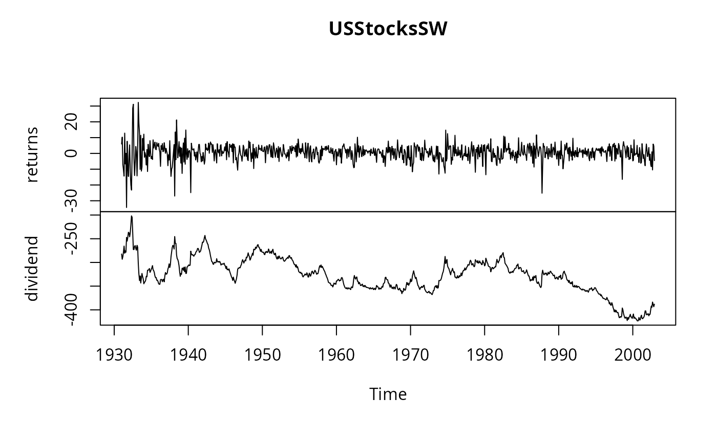
Monthly US Stock Returns (1931–2002, Stock & Watson)

Monthly data from 1931–2002 for US stock prices, measured by the broad-based (NYSE and AMEX) value-weighted index of stock prices as constructed by the Center for Research in Security Prices (CRSP).

Usage

data("USStocksSW")

Format

A monthly multiple time series from 1931(1) to 2002(12) with 2 variables.

returns: monthly excess returns. The monthly return on stocks (in percentage terms) minus the return on a safe asset (in this case: US treasury bill). The return on the stocks includes the price changes plus any dividends you receive during the month.
dividend: 100 times log(dividend yield). (Multiplication by 100 means the changes are interpreted as percentage points). It is calculated as the dividends over the past 12 months, divided by the price in the current month.

Source

Online complements to Stock and Watson (2007).

References

Campbell, J.Y., and Yogo, M. (2006). Efficient Tests of Stock Return Predictability Journal of Financial Economics, 81, 27–60.

Stock, J.H. and Watson, M.W. (2007). Introduction to Econometrics, 2nd ed. Boston: Addison Wesley.

Examples

data("USStocksSW")
plot(USStocksSW)


## Stock and Watson, p. 540, Table 14.3
library("dynlm")
fm1 <- dynlm(returns ~ L(returns), data = USStocksSW, start = c(1960,1))
coeftest(fm1, vcov = sandwich)
#> 
#> t test of coefficients:
#> 
#>             Estimate Std. Error t value Pr(>|t|)
#> (Intercept) 0.311562   0.197371  1.5786   0.1151
#> L(returns)  0.050390   0.051208  0.9840   0.3256
#> 
fm2 <- dynlm(returns ~ L(returns, 1:2), data = USStocksSW, start = c(1960,1))
waldtest(fm2, vcov = sandwich)
#> Wald test
#> 
#> Model 1: returns ~ L(returns, 1:2)
#> Model 2: returns ~ 1
#>   Res.Df Df      F Pr(>F)
#> 1    513                 
#> 2    515 -2 1.3423 0.2622
fm3 <- dynlm(returns ~ L(returns, 1:4), data = USStocksSW, start = c(1960,1))
waldtest(fm3, vcov = sandwich)
#> Wald test
#> 
#> Model 1: returns ~ L(returns, 1:4)
#> Model 2: returns ~ 1
#>   Res.Df Df      F Pr(>F)
#> 1    511                 
#> 2    515 -4 0.7069 0.5875

## Stock and Watson, p. 574, Table 14.7
fm4 <- dynlm(returns ~ L(returns) + L(d(dividend)), data = USStocksSW, start = c(1960, 1))
fm5 <- dynlm(returns ~ L(returns, 1:2) + L(d(dividend), 1:2), data = USStocksSW, start = c(1960,1))
fm6 <- dynlm(returns ~ L(returns) + L(dividend), data = USStocksSW, start = c(1960,1))