Extrapolated Species Richness in a Species Pool
specpool.RdThe functions estimate the extrapolated species richness in a species
pool, or the number of unobserved species. Function specpool
is based on incidences in sample sites, and gives a single estimate
for a collection of sample sites (matrix). Function estimateR
is based on abundances (counts) on single sample site.
Arguments
- x
Data frame or matrix with species data or the analysis result for
plotfunction.- pool
A vector giving a classification for pooling the sites in the species data. If missing, all sites are pooled together.
- smallsample
Use small sample correction \((N-1)/N\), where \(N\) is the number of sites within the
pool.- X, object
A
specpoolresult object.- index
The selected index of extrapolated richness.
- permutations
Usually an integer giving the number permutations, but can also be a list of control values for the permutations as returned by the function
how, or a permutation matrix where each row gives the permuted indices.- parallel
Number of parallel processes or a predefined socket cluster. With
parallel = 1uses ordinary, non-parallel processing. The parallel processing is done with parallel package.- display
Indices to be displayed.
- alpha
Level of quantiles shown. This proportion will be left outside symmetric limits.
- ...
Other parameters (not used).
Details
Many species will always remain unseen or undetected in a collection of sample plots. The function uses some popular ways of estimating the number of these unseen species and adding them to the observed species richness (Palmer 1990, Colwell & Coddington 1994).
The incidence-based estimates in specpool use the frequencies
of species in a collection of sites.
In the following, \(S_P\) is the extrapolated richness in a pool,
\(S_0\) is the observed number of species in the
collection, \(a_1\) and \(a_2\) are the number of species
occurring only in one or only in two sites in the collection, \(p_i\)
is the frequency of species \(i\), and \(N\) is the number of
sites in the collection. The variants of extrapolated richness in
specpool are:
| Chao | \(S_P = S_0 + \frac{a_1^2}{2 a_2}\frac{N-1}{N}\) |
| Chao bias-corrected | \(S_P = S_0 + \frac{a_1(a_1-1)}{2(a_2+1)} \frac{N-1}{N}\) |
| First order jackknife | \(S_P = S_0 + a_1 \frac{N-1}{N}\) |
| Second order jackknife | \(S_P = S_0 + a_1 \frac{2N - 3}{N} - a_2 \frac{(N-2)^2}{N (N-1)}\) |
| Bootstrap | \(S_P = S_0 + \sum_{i=1}^{S_0} (1 - p_i)^N\) |
specpool normally uses basic Chao equation, but when there
are no doubletons (\(a2=0\)) it switches to bias-corrected
version. In that case the Chao equation simplifies to
\(S_0 + \frac{1}{2} a_1 (a_1-1) \frac{N-1}{N}\).
The abundance-based estimates in estimateR use counts
(numbers of individuals) of species in a single site. If called for
a matrix or data frame, the function will give separate estimates
for each site. The two variants of extrapolated richness in
estimateR are bias-corrected Chao and ACE (O'Hara 2005, Chiu
et al. 2014). The Chao estimate is similar as the bias corrected
one above, but \(a_i\) refers to the number of species with
abundance \(i\) instead of number of sites, and the small-sample
correction is not used. The ACE estimate is defined as:
| ACE | \(S_P = S_{abund} + \frac{S_{rare}}{C_{ace}}+ \frac{a_1}{C_{ace}} \gamma^2_{ace}\) |
| where | \(C_{ace} = 1 - \frac{a_1}{N_{rare}}\) |
| \(\gamma^2_{ace} = \max \left[ \frac{S_{rare} \sum_{i=1}^{10} i(i-1)a_i}{C_{ace} N_{rare} (N_{rare} - 1)}-1, 0 \right]\) |
Here \(a_i\) refers to number of species with abundance \(i\) and \(S_{rare}\) is the number of rare species, \(S_{abund}\) is the number of abundant species, with an arbitrary threshold of abundance 10 for rare species, and \(N_{rare}\) is the number of individuals in rare species.
Functions estimate the standard errors of the estimates. These only
concern the number of added species, and assume that there is no
variance in the observed richness. The equations of standard errors
are too complicated to be reproduced in this help page, but they can
be studied in the R source code of the function and are discussed
in the vignette that can be read with the
browseVignettes("vegan"). The standard error are based on the
following sources: Chiu et al. (2014) for the Chao estimates and
Smith and van Belle (1984) for the first-order Jackknife and the
bootstrap (second-order jackknife is still missing). For the
variance estimator of \(S_{ace}\) see O'Hara (2005).
Functions poolaccum and estaccumR are similar to
specaccum, but estimate extrapolated richness indices
of specpool or estimateR in addition to number of
species for random ordering of sampling units. Function
specpool uses presence data and estaccumR count
data. The functions share summary and plot
methods. The summary returns quantile envelopes of
permutations corresponding the given level of alpha and
standard deviation of permutations for each sample size. NB., these
are not based on standard deviations estimated within specpool
or estimateR, but they are based on permutations.
ggvegan provides function autoplot to show the
results of poolaccum.
Value
Function specpool returns a data frame with entries for
observed richness and each of the indices for each class in
pool vector. The utility function specpool2vect maps
the pooled values into a vector giving the value of selected
index for each original site. Function estimateR
returns the estimates and their standard errors for each
site. Functions poolaccum and estimateR return
matrices of permutation results for each richness estimator, the
vector of sample sizes and a table of means of permutations
for each estimator.
References
Chao, A. (1987). Estimating the population size for capture-recapture data with unequal catchability. Biometrics 43, 783–791.
Chiu, C.H., Wang, Y.T., Walther, B.A. & Chao, A. (2014). Improved nonparametric lower bound of species richness via a modified Good-Turing frequency formula. Biometrics 70, 671–682.
Colwell, R.K. & Coddington, J.A. (1994). Estimating terrestrial biodiversity through extrapolation. Phil. Trans. Roy. Soc. London B 345, 101–118.
O'Hara, R.B. (2005). Species richness estimators: how many species can dance on the head of a pin? J. Anim. Ecol. 74, 375–386.
Palmer, M.W. (1990). The estimation of species richness by extrapolation. Ecology 71, 1195–1198.
Smith, E.P & van Belle, G. (1984). Nonparametric estimation of species richness. Biometrics 40, 119–129.
Note
The functions are based on assumption that there is a species pool: The community is closed so that there is a fixed pool size \(S_P\). In general, the functions give only the lower limit of species richness: the real richness is \(S >= S_P\), and there is a consistent bias in the estimates. Even the bias-correction in Chao only reduces the bias, but does not remove it completely (Chiu et al. 2014).
Optional small sample correction was added to specpool in
vegan 2.2-0. It was not used in the older literature (Chao
1987), but it is recommended recently (Chiu et al. 2014).
Examples
data(dune)
data(dune.env)
pool <- with(dune.env, specpool(dune, Management))
pool
#> Species chao chao.se jack1 jack1.se jack2 boot boot.se n
#> BF 16 17.19048 1.5895675 19.33333 2.211083 19.83333 17.74074 1.646379 3
#> HF 21 21.51429 0.9511693 23.40000 1.876166 22.05000 22.56864 1.821518 5
#> NM 21 22.87500 2.1582871 26.00000 3.291403 25.73333 23.77696 2.300982 6
#> SF 21 29.88889 8.6447967 27.66667 3.496029 31.40000 23.99496 1.850288 6
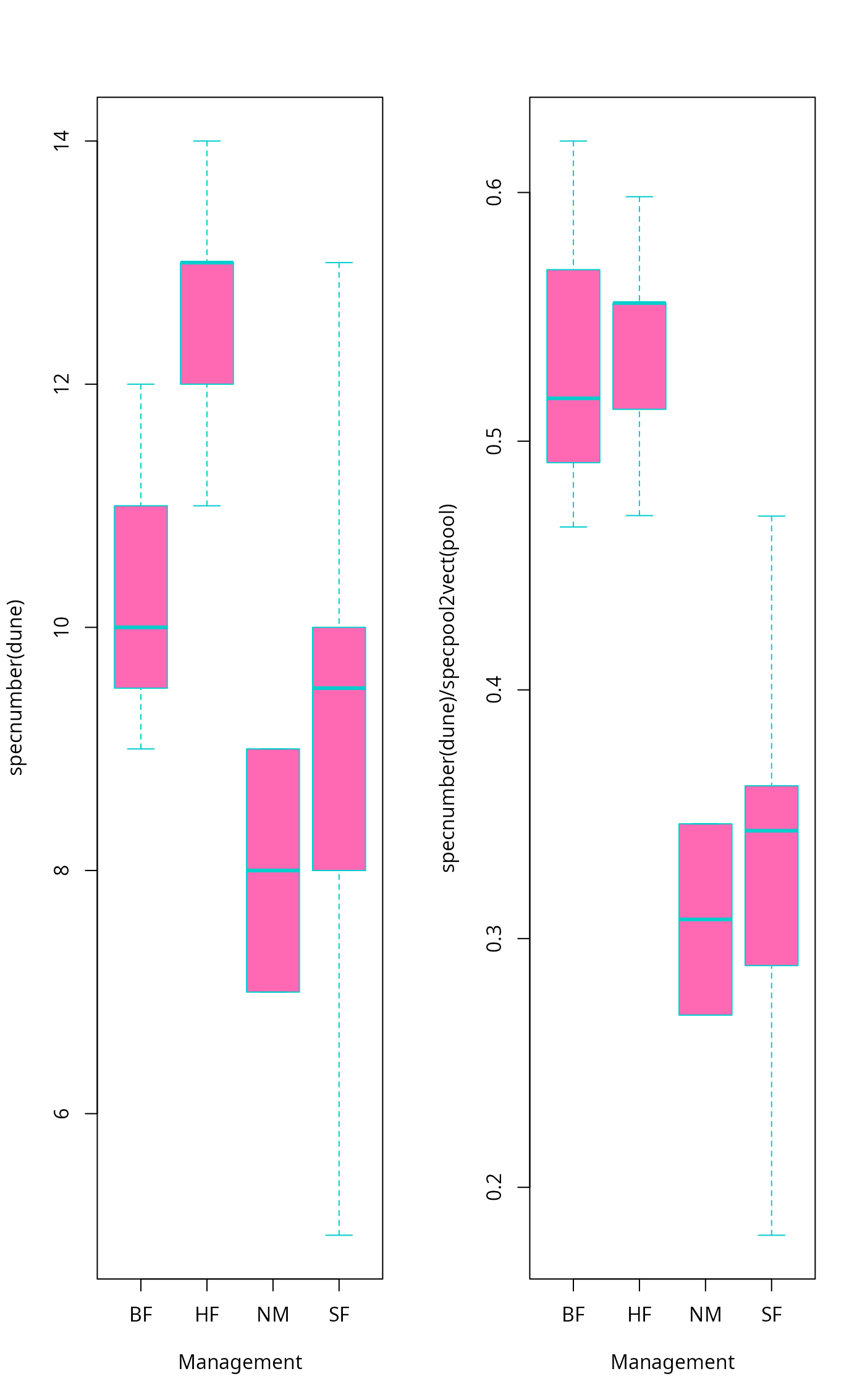
op <- par(mfrow=c(1,2))
boxplot(specnumber(dune) ~ Management, data = dune.env,
col = "hotpink", border = "cyan3")
boxplot(specnumber(dune)/specpool2vect(pool) ~ Management,
data = dune.env, col = "hotpink", border = "cyan3")
 par(op)
data(BCI)
## Accumulation model
pool <- poolaccum(BCI)
summary(pool, display = "chao")
#> $chao
#> N Chao 2.5% 97.5% Std.Dev
#> [1,] 3 162.4962 144.1768 184.6034 11.013673
#> [2,] 4 175.0666 158.5404 198.7598 10.336065
#> [3,] 5 183.2328 163.5337 205.0909 11.257256
#> [4,] 6 189.7016 168.6770 208.7810 10.732083
#> [5,] 7 194.2132 172.3986 215.6655 11.374111
#> [6,] 8 197.9736 177.9252 223.3080 11.910751
#> [7,] 9 202.5775 182.1626 231.4184 12.177899
#> [8,] 10 204.9109 187.4196 227.2824 10.499770
#> [9,] 11 207.6703 188.3662 233.7068 12.111882
#> [10,] 12 210.3659 191.9714 237.4984 12.490919
#> [11,] 13 212.7621 191.8792 238.3554 12.130824
#> [12,] 14 214.7277 194.3292 235.3735 11.490910
#> [13,] 15 216.7219 196.5686 237.6484 10.816425
#> [14,] 16 218.8620 196.6856 241.9348 11.454730
#> [15,] 17 220.4776 200.2000 243.2424 11.588090
#> [16,] 18 222.6102 200.8186 248.0647 12.490470
#> [17,] 19 224.1822 205.7467 251.1151 14.662874
#> [18,] 20 225.9782 207.8935 251.0283 12.687050
#> [19,] 21 227.8953 208.2949 253.7712 13.951917
#> [20,] 22 229.3368 211.3295 252.6615 12.531505
#> [21,] 23 230.0760 212.8913 262.0005 12.535490
#> [22,] 24 232.0528 214.2676 261.9333 12.266608
#> [23,] 25 233.5858 215.2900 262.8136 12.836894
#> [24,] 26 235.2666 214.7191 264.9190 13.693366
#> [25,] 27 236.6923 216.7275 260.7063 13.868347
#> [26,] 28 236.8844 216.4915 263.7886 13.343042
#> [27,] 29 236.7143 216.6731 265.5569 13.312264
#> [28,] 30 237.2034 219.1378 268.0749 12.736071
#> [29,] 31 237.3492 220.0248 264.4282 12.624476
#> [30,] 32 237.5144 219.5750 265.1425 11.364696
#> [31,] 33 237.4255 220.6891 263.9819 10.371750
#> [32,] 34 237.8840 222.7996 263.1415 10.501549
#> [33,] 35 237.4282 223.7120 261.9086 9.707338
#> [34,] 36 237.4848 223.8337 255.9057 9.478582
#> [35,] 37 236.5480 225.6721 254.0547 8.380387
#> [36,] 38 236.3995 225.6577 257.2428 8.339691
#> [37,] 39 237.2985 225.0141 259.5813 8.605379
#> [38,] 40 236.9973 225.7060 252.1612 7.580101
#> [39,] 41 237.2854 225.4600 252.5086 7.503844
#> [40,] 42 237.4214 224.5666 253.9669 7.603727
#> [41,] 43 237.2858 226.0694 253.9841 7.320998
#> [42,] 44 237.4748 226.3584 254.3531 6.874040
#> [43,] 45 237.0024 226.3900 254.2483 6.149373
#> [44,] 46 237.0589 227.6179 252.4475 5.390659
#> [45,] 47 237.1238 229.3398 252.4419 5.139588
#> [46,] 48 236.4255 231.1027 246.2732 3.539775
#> [47,] 49 236.3515 231.3403 242.9539 2.428696
#> [48,] 50 236.3732 236.3732 236.3732 0.000000
#>
#> attr(,"class")
#> [1] "summary.poolaccum"
## Quantitative model
estimateR(BCI[1:5,])
#> 1 2 3 4 5
#> S.obs 93.000000 84.000000 90.000000 94.000000 101.000000
#> S.chao1 117.473684 117.214286 141.230769 111.550000 136.000000
#> se.chao1 11.583785 15.918953 23.001405 8.919663 15.467344
#> S.ACE 122.848959 117.317307 134.669844 118.729941 137.114088
#> se.ACE 5.736054 5.571998 6.191618 5.367571 5.848474
par(op)
data(BCI)
## Accumulation model
pool <- poolaccum(BCI)
summary(pool, display = "chao")
#> $chao
#> N Chao 2.5% 97.5% Std.Dev
#> [1,] 3 162.4962 144.1768 184.6034 11.013673
#> [2,] 4 175.0666 158.5404 198.7598 10.336065
#> [3,] 5 183.2328 163.5337 205.0909 11.257256
#> [4,] 6 189.7016 168.6770 208.7810 10.732083
#> [5,] 7 194.2132 172.3986 215.6655 11.374111
#> [6,] 8 197.9736 177.9252 223.3080 11.910751
#> [7,] 9 202.5775 182.1626 231.4184 12.177899
#> [8,] 10 204.9109 187.4196 227.2824 10.499770
#> [9,] 11 207.6703 188.3662 233.7068 12.111882
#> [10,] 12 210.3659 191.9714 237.4984 12.490919
#> [11,] 13 212.7621 191.8792 238.3554 12.130824
#> [12,] 14 214.7277 194.3292 235.3735 11.490910
#> [13,] 15 216.7219 196.5686 237.6484 10.816425
#> [14,] 16 218.8620 196.6856 241.9348 11.454730
#> [15,] 17 220.4776 200.2000 243.2424 11.588090
#> [16,] 18 222.6102 200.8186 248.0647 12.490470
#> [17,] 19 224.1822 205.7467 251.1151 14.662874
#> [18,] 20 225.9782 207.8935 251.0283 12.687050
#> [19,] 21 227.8953 208.2949 253.7712 13.951917
#> [20,] 22 229.3368 211.3295 252.6615 12.531505
#> [21,] 23 230.0760 212.8913 262.0005 12.535490
#> [22,] 24 232.0528 214.2676 261.9333 12.266608
#> [23,] 25 233.5858 215.2900 262.8136 12.836894
#> [24,] 26 235.2666 214.7191 264.9190 13.693366
#> [25,] 27 236.6923 216.7275 260.7063 13.868347
#> [26,] 28 236.8844 216.4915 263.7886 13.343042
#> [27,] 29 236.7143 216.6731 265.5569 13.312264
#> [28,] 30 237.2034 219.1378 268.0749 12.736071
#> [29,] 31 237.3492 220.0248 264.4282 12.624476
#> [30,] 32 237.5144 219.5750 265.1425 11.364696
#> [31,] 33 237.4255 220.6891 263.9819 10.371750
#> [32,] 34 237.8840 222.7996 263.1415 10.501549
#> [33,] 35 237.4282 223.7120 261.9086 9.707338
#> [34,] 36 237.4848 223.8337 255.9057 9.478582
#> [35,] 37 236.5480 225.6721 254.0547 8.380387
#> [36,] 38 236.3995 225.6577 257.2428 8.339691
#> [37,] 39 237.2985 225.0141 259.5813 8.605379
#> [38,] 40 236.9973 225.7060 252.1612 7.580101
#> [39,] 41 237.2854 225.4600 252.5086 7.503844
#> [40,] 42 237.4214 224.5666 253.9669 7.603727
#> [41,] 43 237.2858 226.0694 253.9841 7.320998
#> [42,] 44 237.4748 226.3584 254.3531 6.874040
#> [43,] 45 237.0024 226.3900 254.2483 6.149373
#> [44,] 46 237.0589 227.6179 252.4475 5.390659
#> [45,] 47 237.1238 229.3398 252.4419 5.139588
#> [46,] 48 236.4255 231.1027 246.2732 3.539775
#> [47,] 49 236.3515 231.3403 242.9539 2.428696
#> [48,] 50 236.3732 236.3732 236.3732 0.000000
#>
#> attr(,"class")
#> [1] "summary.poolaccum"
## Quantitative model
estimateR(BCI[1:5,])
#> 1 2 3 4 5
#> S.obs 93.000000 84.000000 90.000000 94.000000 101.000000
#> S.chao1 117.473684 117.214286 141.230769 111.550000 136.000000
#> se.chao1 11.583785 15.918953 23.001405 8.919663 15.467344
#> S.ACE 122.848959 117.317307 134.669844 118.729941 137.114088
#> se.ACE 5.736054 5.571998 6.191618 5.367571 5.848474