Species Accumulation Curves
specaccum.RdFunction specaccum finds species accumulation curves or the
number of species for a certain number of sampled sites or
individuals.
Usage
specaccum(comm, method = "exact", permutations = 100,
          conditioned =TRUE, gamma = "jack1",  w = NULL, subset, ...)
# S3 method for class 'specaccum'
plot(x, add = FALSE, random = FALSE, ci = 2,
    ci.type = c("bar", "line", "polygon"), col = par("fg"), lty = 1,
    ci.col = col, ci.lty = 1, ci.length = 0, xlab, ylab = x$method, ylim,
    xvar = c("sites", "individuals", "effort"), ...)
# S3 method for class 'specaccum'
boxplot(x, add = FALSE, ...)
fitspecaccum(object, model, method = "random", ...)
# S3 method for class 'fitspecaccum'
plot(x, col = par("fg"), lty = 1, xlab = "Sites",
    ylab = x$method, ...)
# S3 method for class 'specaccum'
predict(object, newdata, interpolation = c("linear", "spline"), ...)
# S3 method for class 'fitspecaccum'
predict(object, newdata, ...)
specslope(object, at)
Arguments
- comm
Community data set.
- method
Species accumulation method (partial match). Method
"collector"adds sites in the order they happen to be in the data,"random"adds sites in random order,"exact"finds the expected (mean) species richness,"coleman"finds the expected richness following Coleman et al. 1982, and"rarefaction"finds the mean when accumulating individuals instead of sites.- permutations
Number of permutations with
method = "random". Usually an integer giving the number permutations, but can also be a list of control values for the permutations as returned by the functionhow, or a permutation matrix where each row gives the permuted indices.- conditioned
Estimation of standard deviation is conditional on the empirical dataset for the exact SAC
- gamma
Method for estimating the total extrapolated number of species in the survey area by function
specpool- w
Weights giving the sampling effort.
- subset
logical expression indicating sites (rows) to keep: missing values are taken as
FALSE.- x
A
specaccumresult object- add
Add to an existing graph.
- random
Draw each random simulation separately instead of drawing their average and confidence intervals.
- ci
Multiplier used to get confidence intervals from standard deviation (standard error of the estimate). Value
ci = 0suppresses drawing confidence intervals.- ci.type
Type of confidence intervals in the graph:
"bar"draws vertical bars,"line"draws lines, and"polygon"draws a shaded area.- col
Colour for drawing lines.
- lty
line type (see
par).- ci.col
Colour for drawing lines or filling the
"polygon".- ci.lty
Line type for confidence intervals or border of the
"polygon".- ci.length
Length of horizontal bars (in inches) at the end of vertical bars with
ci.type = "bar".- xlab,ylab
Labels for
x(defaultsxvar) andyaxis.- ylim
the y limits of the plot.
- xvar
Variable used for the horizontal axis:
"individuals"can be used only withmethod = "rarefaction".- object
Either a community data set or fitted
specaccummodel.- model
Nonlinear regression model (
nls). See Details.- newdata
Optional data used in prediction interpreted as number of sampling units (sites). If missing, fitted values are returned.
- interpolation
Interpolation method used with
newdata.- at
Number of plots where the slope is evaluated. Can be a real number.
- ...
Other parameters to functions.
Details
Species accumulation curves (SAC) are used to compare diversity
properties of community data sets using different accumulator
functions. The classic method is "random" which finds the mean
SAC and its standard deviation from random permutations of the data,
or subsampling without replacement (Gotelli & Colwell 2001). The
"exact" method finds the expected SAC using sample-based
rarefaction method that has been independently developed numerous
times (Chiarucci et al. 2008) and it is often known as Mao Tau
estimate (Colwell et al. 2012). The unconditional standard deviation
for the exact SAC represents a moment-based estimation that is not
conditioned on the empirical data set (sd for all samples > 0). The
unconditional standard deviation is based on an estimation of the
extrapolated number of species in the survey area (a.k.a. gamma
diversity), as estimated by function specpool. The
conditional standard deviation that was developed by Jari Oksanen (not
published, sd=0 for all samples). Method "coleman" finds the
expected SAC and its standard deviation following Coleman et
al. (1982). All these methods are based on sampling sites without
replacement. In contrast, the method = "rarefaction" finds the
expected species richness and its standard deviation by sampling
individuals instead of sites. It achieves this by applying function
rarefy with number of individuals corresponding to
average number of individuals per site.
Methods "random" and "collector" can take weights
(w) that give the sampling effort for each site. The weights
w do not influence the order the sites are accumulated, but
only the value of the sampling effort so that not all sites are
equal. The summary results are expressed against sites even when the
accumulation uses weights (methods "random",
"collector"), or is based on individuals
("rarefaction"). The actual sampling effort is given as item
Effort or Individuals in the printed result. For
weighted "random" method the effort refers to the average
effort per site, or sum of weights per number of sites. With
weighted method = "random", the averaged species richness is
found from linear interpolation of single random permutations.
Therefore at least the first value (and often several first) have
NA richness, because these values cannot be interpolated in
all cases but should be extrapolated. The plot function
defaults to display the results as scaled to sites, but this can be
changed selecting xvar = "effort" (weighted methods) or
xvar = "individuals" (with method = "rarefaction").
The summary and boxplot methods are available for
method = "random".
Function predict for specaccum can return the values
corresponding to newdata. With method "exact",
"rarefaction" and "coleman" the function uses analytic
equations for interpolated non-integer values, and for other methods
linear (approx) or spline (spline)
interpolation. If newdata is not given, the function returns
the values corresponding to the data. NB., the fitted values with
method="rarefaction" are based on rounded integer counts, but
predict can use fractional non-integer counts with
newdata and give slightly different results.
Function fitspecaccum fits a nonlinear (nls)
self-starting species accumulation model. The input object
can be a result of specaccum or a community in data frame. In
the latter case the function first fits a specaccum model and
then proceeds with fitting the nonlinear model. The function can
apply a limited set of nonlinear regression models suggested for
species-area relationship (Dengler 2009). All these are
selfStart models. The permissible alternatives are
"arrhenius" (SSarrhenius), "gleason"
(SSgleason), "gitay" (SSgitay),
"lomolino" (SSlomolino) of vegan
package. In addition the following standard R models are available:
"asymp" (SSasymp), "gompertz"
(SSgompertz), "michaelis-menten"
(SSmicmen), "logis" (SSlogis),
"weibull" (SSweibull). See these functions for
model specification and details.
When weights w were used the fit is based on accumulated
effort and in model = "rarefaction" on accumulated number of
individuals. The plot is still based on sites, unless other
alternative is selected with xvar.
Function predict for fitspecaccum uses
predict.nls, and you can pass all arguments to that
function. In addition, fitted, residuals, nobs,
coef, AIC, logLik and deviance work on
the result object.
Function specslope evaluates the derivative of the species
accumulation curve at given number of sample plots, and gives the
rate of increase in the number of species. The function works with
specaccum result object when this is based on analytic models
"exact", "rarefaction" or "coleman", and with
non-linear regression results of fitspecaccum.
Nonlinear regression may fail for any reason, and some of the
fitspecaccum models are fragile and may not succeed.
Value
Function specaccum returns an object of class
"specaccum", and fitspecaccum a model of class
"fitspecaccum" that adds a few items to the
"specaccum" (see the end of the list below):
- call
Function call.
- method
Accumulator method.
- sites
Number of sites. For
method = "rarefaction"this is the number of sites corresponding to a certain number of individuals and generally not an integer, and the average number of individuals is also returned in itemindividuals.- effort
Average sum of weights corresponding to the number of sites when model was fitted with argument
w- richness
The number of species corresponding to number of sites. With
method = "collector"this is the observed richness, for other methods the average or expected richness.- sd
The standard deviation of SAC (or its standard error). This is
NULLinmethod = "collector", and it is estimated from permutations inmethod = "random", and from analytic equations in other methods.- perm
Permutation results with
method = "random"andNULLin other cases. Each column inpermholds one permutation.- weights
Matrix of accumulated weights corresponding to the columns of the
permmatrix when model was fitted with argumentw.- fitted, residuals, coefficients
Only in
fitspecacum: fitted values, residuals and nonlinear model coefficients. Formethod = "random"these are matrices with a column for each random accumulation.- models
Only in
fitspecaccum: list of fittednlsmodels (see Examples on accessing these models).
References
Chiarucci, A., Bacaro, G., Rocchini, D. & Fattorini, L. (2008). Discovering and rediscovering the sample-based rarefaction formula in the ecological literature. Commun. Ecol. 9: 121–123.
Coleman, B.D, Mares, M.A., Willis, M.R. & Hsieh, Y. (1982). Randomness, area and species richness. Ecology 63: 1121–1133.
Colwell, R.K., Chao, A., Gotelli, N.J., Lin, S.Y., Mao, C.X., Chazdon, R.L. & Longino, J.T. (2012). Models and estimators linking individual-based and sample-based rarefaction, extrapolation and comparison of assemblages. J. Plant Ecol. 5: 3–21.
Dengler, J. (2009). Which function describes the species-area relationship best? A review and empirical evaluation. Journal of Biogeography 36, 728–744.
Gotelli, N.J. & Colwell, R.K. (2001). Quantifying biodiversity: procedures and pitfalls in measurement and comparison of species richness. Ecol. Lett. 4, 379–391.
Author
Roeland Kindt r.kindt@cgiar.org and Jari Oksanen.
Note
The SAC with method = "exact" was
developed by Roeland Kindt, and its standard deviation by Jari
Oksanen (both are unpublished). The method = "coleman"
underestimates the SAC because it does not handle properly sampling
without replacement. Further, its standard deviation does not take
into account species correlations, and is generally too low.
See also
rarefy and rrarefy are related
individual based models. Other accumulation models are
poolaccum for extrapolated richness, and
renyiaccum and tsallisaccum for
diversity indices. Underlying graphical functions are
boxplot, matlines,
segments and polygon.
Examples
data(BCI)
sp1 <- specaccum(BCI)
#> Warning: the standard deviation is zero
sp2 <- specaccum(BCI, "random")
sp2
#> Species Accumulation Curve
#> Accumulation method: random, with 100 permutations
#> Call: specaccum(comm = BCI, method = "random")
#>
#>
#> Sites 1.00000 2.0000 3.00000 4.00000 5.00000 6.00000 7.000
#> Richness 90.82000 122.3500 138.86000 150.93000 159.37000 166.08000 171.670
#> sd 7.40922 7.1934 6.65456 6.31537 6.16549 5.30233 5.111
#>
#> Sites 8.00000 9.00000 10.00000 11.00000 12.00000 13.00000 14.00000
#> Richness 175.61000 179.27000 182.59000 185.54000 188.15000 190.34000 192.25000
#> sd 5.05504 5.06494 4.75266 4.66108 4.54689 4.56429 4.22684
#>
#> Sites 15.00000 16.00000 17.00000 18.00000 19.00000 20.00000 21.00000
#> Richness 194.27000 195.99000 197.75000 199.31000 200.78000 202.29000 203.64000
#> sd 4.08212 3.97338 3.72644 3.87349 3.65032 3.61337 3.40683
#>
#> Sites 22.0000 23.00000 24.00000 25.0000 26.00000 27.00000 28.00000
#> Richness 204.9200 206.14000 207.27000 208.2800 209.39000 210.32000 211.27000
#> sd 3.4951 3.55624 3.63445 3.5193 3.37218 3.29334 3.25935
#>
#> Sites 29.00000 30.00000 31.00000 32.00000 33.00000 34.0000 35.00000
#> Richness 212.03000 212.97000 213.76000 214.46000 215.24000 215.9800 216.63000
#> sd 3.16373 2.94205 2.96144 2.81561 2.61356 2.7413 2.65777
#>
#> Sites 36.00000 37.0000 38.00000 39.0000 40.00000 41.00000 42.00000
#> Richness 217.42000 218.0200 218.67000 219.3200 220.00000 220.60000 221.07000
#> sd 2.61379 2.4984 2.36581 2.3393 2.11297 1.98479 1.84366
#>
#> Sites 43.00000 44.0000 45.0000 46.00000 47.00000 48.00000 49.00000
#> Richness 221.47000 222.0800 222.6500 223.35000 223.76000 224.18000 224.65000
#> sd 1.76644 1.6738 1.4521 1.25025 1.12025 0.96797 0.64157
#>
#> Sites 50
#> Richness 225
#> sd 0
summary(sp2)
#> 1 sites 2 sites 3 sites 4 sites
#> Min. : 77.00 Min. :105.0 Min. :124.0 Min. :137.0
#> 1st Qu.: 86.00 1st Qu.:118.0 1st Qu.:135.0 1st Qu.:147.0
#> Median : 91.00 Median :122.0 Median :139.0 Median :151.0
#> Mean : 90.82 Mean :122.3 Mean :138.9 Mean :150.9
#> 3rd Qu.: 97.25 3rd Qu.:127.0 3rd Qu.:143.2 3rd Qu.:155.0
#> Max. :109.00 Max. :139.0 Max. :154.0 Max. :164.0
#> 5 sites 6 sites 7 sites 8 sites
#> Min. :143.0 Min. :156.0 Min. :161.0 Min. :164.0
#> 1st Qu.:156.0 1st Qu.:162.0 1st Qu.:168.0 1st Qu.:172.0
#> Median :160.0 Median :166.0 Median :172.0 Median :175.0
#> Mean :159.4 Mean :166.1 Mean :171.7 Mean :175.6
#> 3rd Qu.:163.2 3rd Qu.:170.0 3rd Qu.:175.2 3rd Qu.:179.0
#> Max. :172.0 Max. :175.0 Max. :183.0 Max. :188.0
#> 9 sites 10 sites 11 sites 12 sites
#> Min. :168.0 Min. :172.0 Min. :177.0 Min. :178.0
#> 1st Qu.:175.0 1st Qu.:179.0 1st Qu.:182.0 1st Qu.:185.0
#> Median :179.0 Median :183.0 Median :186.0 Median :188.0
#> Mean :179.3 Mean :182.6 Mean :185.5 Mean :188.2
#> 3rd Qu.:183.0 3rd Qu.:186.0 3rd Qu.:189.0 3rd Qu.:192.0
#> Max. :192.0 Max. :195.0 Max. :198.0 Max. :201.0
#> 13 sites 14 sites 15 sites 16 sites 17 sites
#> Min. :181.0 Min. :182.0 Min. :183.0 Min. :186 Min. :188.0
#> 1st Qu.:187.0 1st Qu.:189.8 1st Qu.:191.8 1st Qu.:193 1st Qu.:195.0
#> Median :190.0 Median :192.0 Median :195.0 Median :196 Median :198.0
#> Mean :190.3 Mean :192.2 Mean :194.3 Mean :196 Mean :197.8
#> 3rd Qu.:193.2 3rd Qu.:195.0 3rd Qu.:197.0 3rd Qu.:199 3rd Qu.:200.0
#> Max. :203.0 Max. :203.0 Max. :204.0 Max. :206 Max. :207.0
#> 18 sites 19 sites 20 sites 21 sites
#> Min. :189.0 Min. :191.0 Min. :193.0 Min. :194.0
#> 1st Qu.:197.0 1st Qu.:199.0 1st Qu.:200.0 1st Qu.:202.0
#> Median :199.0 Median :201.0 Median :202.0 Median :204.0
#> Mean :199.3 Mean :200.8 Mean :202.3 Mean :203.6
#> 3rd Qu.:202.0 3rd Qu.:203.0 3rd Qu.:204.0 3rd Qu.:205.2
#> Max. :210.0 Max. :211.0 Max. :212.0 Max. :212.0
#> 22 sites 23 sites 24 sites 25 sites
#> Min. :195.0 Min. :195.0 Min. :196.0 Min. :197.0
#> 1st Qu.:203.0 1st Qu.:204.0 1st Qu.:205.0 1st Qu.:206.0
#> Median :205.0 Median :206.0 Median :207.0 Median :208.0
#> Mean :204.9 Mean :206.1 Mean :207.3 Mean :208.3
#> 3rd Qu.:207.0 3rd Qu.:208.2 3rd Qu.:210.0 3rd Qu.:211.0
#> Max. :214.0 Max. :216.0 Max. :216.0 Max. :217.0
#> 26 sites 27 sites 28 sites 29 sites 30 sites
#> Min. :202.0 Min. :203.0 Min. :204.0 Min. :205 Min. :206
#> 1st Qu.:207.0 1st Qu.:208.0 1st Qu.:209.0 1st Qu.:210 1st Qu.:211
#> Median :209.0 Median :210.0 Median :211.0 Median :212 Median :213
#> Mean :209.4 Mean :210.3 Mean :211.3 Mean :212 Mean :213
#> 3rd Qu.:212.0 3rd Qu.:212.0 3rd Qu.:213.0 3rd Qu.:214 3rd Qu.:215
#> Max. :219.0 Max. :219.0 Max. :220.0 Max. :220 Max. :220
#> 31 sites 32 sites 33 sites 34 sites 35 sites
#> Min. :207.0 Min. :208.0 Min. :210.0 Min. :210 Min. :210.0
#> 1st Qu.:212.0 1st Qu.:213.0 1st Qu.:213.8 1st Qu.:214 1st Qu.:215.0
#> Median :214.0 Median :214.0 Median :215.0 Median :216 Median :217.0
#> Mean :213.8 Mean :214.5 Mean :215.2 Mean :216 Mean :216.6
#> 3rd Qu.:216.0 3rd Qu.:216.0 3rd Qu.:217.0 3rd Qu.:218 3rd Qu.:218.2
#> Max. :221.0 Max. :222.0 Max. :222.0 Max. :223 Max. :224.0
#> 36 sites 37 sites 38 sites 39 sites 40 sites
#> Min. :210.0 Min. :210.0 Min. :212.0 Min. :213.0 Min. :215
#> 1st Qu.:216.0 1st Qu.:217.0 1st Qu.:217.8 1st Qu.:218.0 1st Qu.:219
#> Median :217.0 Median :218.0 Median :219.0 Median :219.5 Median :220
#> Mean :217.4 Mean :218.0 Mean :218.7 Mean :219.3 Mean :220
#> 3rd Qu.:219.0 3rd Qu.:219.2 3rd Qu.:220.0 3rd Qu.:221.0 3rd Qu.:221
#> Max. :224.0 Max. :224.0 Max. :224.0 Max. :225.0 Max. :225
#> 41 sites 42 sites 43 sites 44 sites
#> Min. :215.0 Min. :215.0 Min. :217.0 Min. :218.0
#> 1st Qu.:220.0 1st Qu.:220.0 1st Qu.:220.0 1st Qu.:221.0
#> Median :221.0 Median :221.0 Median :222.0 Median :222.0
#> Mean :220.6 Mean :221.1 Mean :221.5 Mean :222.1
#> 3rd Qu.:222.0 3rd Qu.:222.0 3rd Qu.:223.0 3rd Qu.:223.0
#> Max. :225.0 Max. :225.0 Max. :225.0 Max. :225.0
#> 45 sites 46 sites 47 sites 48 sites
#> Min. :219.0 Min. :220.0 Min. :221.0 Min. :221.0
#> 1st Qu.:222.0 1st Qu.:223.0 1st Qu.:223.0 1st Qu.:224.0
#> Median :223.0 Median :224.0 Median :224.0 Median :224.0
#> Mean :222.7 Mean :223.3 Mean :223.8 Mean :224.2
#> 3rd Qu.:224.0 3rd Qu.:224.0 3rd Qu.:225.0 3rd Qu.:225.0
#> Max. :225.0 Max. :225.0 Max. :225.0 Max. :225.0
#> 49 sites 50 sites
#> Min. :222.0 Min. :225
#> 1st Qu.:224.0 1st Qu.:225
#> Median :225.0 Median :225
#> Mean :224.7 Mean :225
#> 3rd Qu.:225.0 3rd Qu.:225
#> Max. :225.0 Max. :225
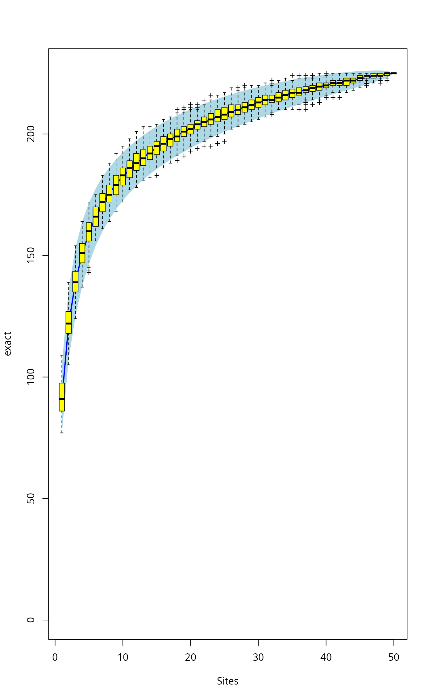
plot(sp1, ci.type="poly", col="blue", lwd=2, ci.lty=0, ci.col="lightblue")
boxplot(sp2, col="yellow", add=TRUE, pch="+")
 ## Fit Lomolino model to the exact accumulation
mod1 <- fitspecaccum(sp1, "lomolino")
coef(mod1)
#> Asym xmid slope
#> 258.440682 2.442061 1.858694
fitted(mod1)
#> [1] 94.34749 121.23271 137.45031 148.83053 157.45735 164.31866 169.95946
#> [8] 174.71115 178.78954 182.34254 185.47566 188.26658 190.77402 193.04337
#> [15] 195.11033 197.00350 198.74606 200.35705 201.85227 203.24499 204.54643
#> [22] 205.76612 206.91229 207.99203 209.01150 209.97609 210.89054 211.75903
#> [29] 212.58527 213.37256 214.12386 214.84180 215.52877 216.18692 216.81820
#> [36] 217.42437 218.00703 218.56767 219.10762 219.62811 220.13027 220.61514
#> [43] 221.08369 221.53679 221.97528 222.39991 222.81138 223.21037 223.59747
#> [50] 223.97327
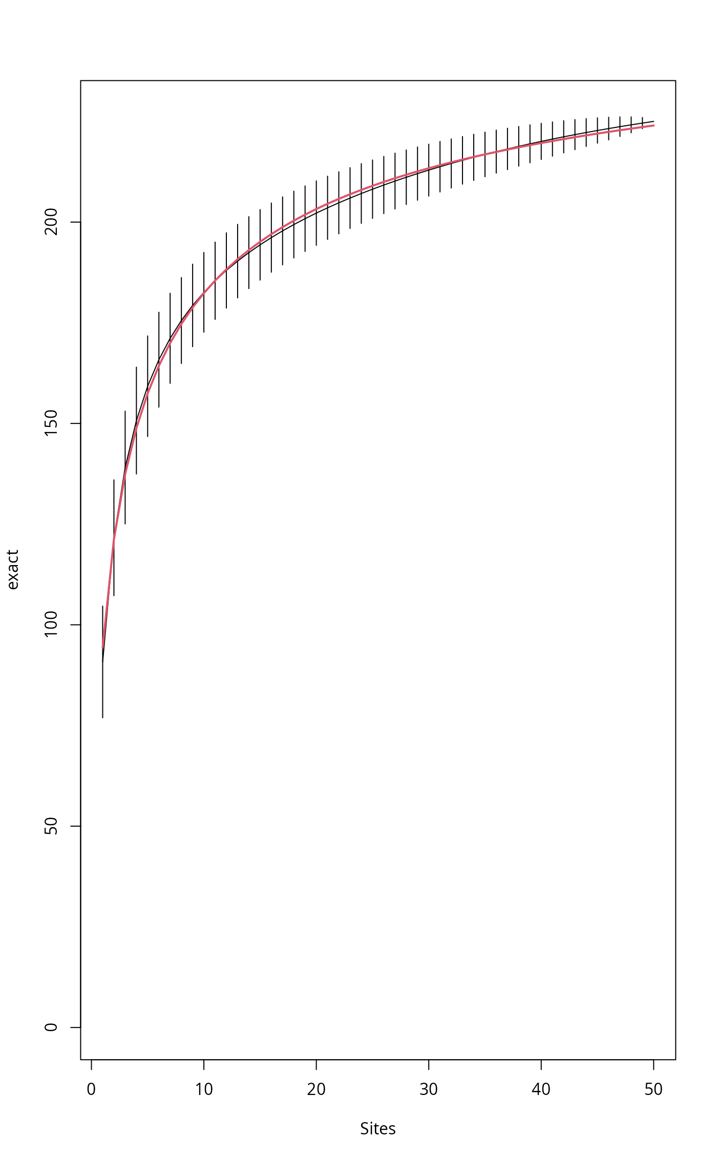
plot(sp1)
## Add Lomolino model using argument 'add'
plot(mod1, add = TRUE, col=2, lwd=2)
## Fit Lomolino model to the exact accumulation
mod1 <- fitspecaccum(sp1, "lomolino")
coef(mod1)
#> Asym xmid slope
#> 258.440682 2.442061 1.858694
fitted(mod1)
#> [1] 94.34749 121.23271 137.45031 148.83053 157.45735 164.31866 169.95946
#> [8] 174.71115 178.78954 182.34254 185.47566 188.26658 190.77402 193.04337
#> [15] 195.11033 197.00350 198.74606 200.35705 201.85227 203.24499 204.54643
#> [22] 205.76612 206.91229 207.99203 209.01150 209.97609 210.89054 211.75903
#> [29] 212.58527 213.37256 214.12386 214.84180 215.52877 216.18692 216.81820
#> [36] 217.42437 218.00703 218.56767 219.10762 219.62811 220.13027 220.61514
#> [43] 221.08369 221.53679 221.97528 222.39991 222.81138 223.21037 223.59747
#> [50] 223.97327
plot(sp1)
## Add Lomolino model using argument 'add'
plot(mod1, add = TRUE, col=2, lwd=2)
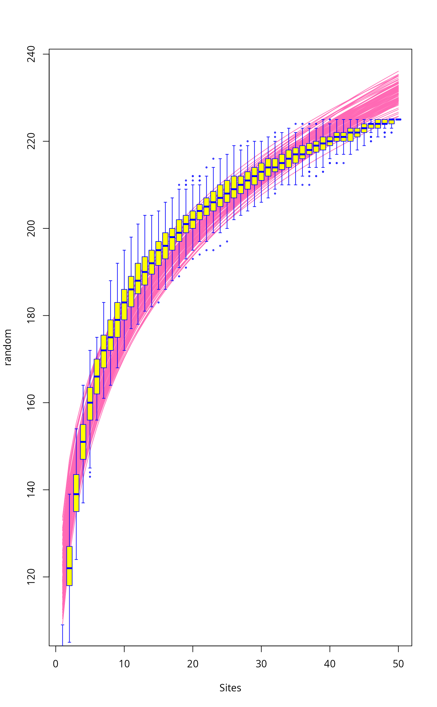
 ## Fit Arrhenius models to all random accumulations
mods <- fitspecaccum(sp2, "arrh")
plot(mods, col="hotpink")
boxplot(sp2, col = "yellow", border = "blue", lty=1, cex=0.3, add= TRUE)
## Fit Arrhenius models to all random accumulations
mods <- fitspecaccum(sp2, "arrh")
plot(mods, col="hotpink")
boxplot(sp2, col = "yellow", border = "blue", lty=1, cex=0.3, add= TRUE)
 ## Use nls() methods to the list of models
sapply(mods$models, AIC)
#> [1] 286.8961 351.7838 332.3137 340.3264 340.3771 339.7776 311.3658 357.4003
#> [9] 325.0910 325.8431 308.3152 322.3239 332.0212 329.0088 307.0817 339.6898
#> [17] 306.4173 315.8755 297.7274 340.2392 325.7479 320.8370 339.8012 290.7299
#> [25] 327.3928 328.3710 328.8589 299.1649 295.2841 344.5453 346.4864 362.9746
#> [33] 344.0147 275.2114 370.7042 325.2480 332.4997 312.4414 330.4092 350.7129
#> [41] 304.6665 316.1088 347.8848 308.3892 351.3432 340.3668 297.0766 338.3913
#> [49] 349.5025 317.4499 311.7487 338.5099 326.3795 336.9187 327.7249 352.8915
#> [57] 329.2000 321.8194 309.8682 332.7265 335.3696 342.3049 349.4023 295.0378
#> [65] 335.3567 356.7021 342.6430 328.4580 327.5102 310.1210 311.2499 311.9706
#> [73] 354.9492 357.2030 338.0017 361.3667 366.0461 312.4395 316.1461 336.2027
#> [81] 330.7645 347.5582 366.2146 347.8397 353.9612 318.8787 355.9027 349.2560
#> [89] 340.2121 327.7220 345.3082 340.9499 335.6730 340.3947 313.4887 295.2562
#> [97] 338.4193 341.9489 383.6567 339.2980
## Use nls() methods to the list of models
sapply(mods$models, AIC)
#> [1] 286.8961 351.7838 332.3137 340.3264 340.3771 339.7776 311.3658 357.4003
#> [9] 325.0910 325.8431 308.3152 322.3239 332.0212 329.0088 307.0817 339.6898
#> [17] 306.4173 315.8755 297.7274 340.2392 325.7479 320.8370 339.8012 290.7299
#> [25] 327.3928 328.3710 328.8589 299.1649 295.2841 344.5453 346.4864 362.9746
#> [33] 344.0147 275.2114 370.7042 325.2480 332.4997 312.4414 330.4092 350.7129
#> [41] 304.6665 316.1088 347.8848 308.3892 351.3432 340.3668 297.0766 338.3913
#> [49] 349.5025 317.4499 311.7487 338.5099 326.3795 336.9187 327.7249 352.8915
#> [57] 329.2000 321.8194 309.8682 332.7265 335.3696 342.3049 349.4023 295.0378
#> [65] 335.3567 356.7021 342.6430 328.4580 327.5102 310.1210 311.2499 311.9706
#> [73] 354.9492 357.2030 338.0017 361.3667 366.0461 312.4395 316.1461 336.2027
#> [81] 330.7645 347.5582 366.2146 347.8397 353.9612 318.8787 355.9027 349.2560
#> [89] 340.2121 327.7220 345.3082 340.9499 335.6730 340.3947 313.4887 295.2562
#> [97] 338.4193 341.9489 383.6567 339.2980