Plots for survey data

Because observations in survey samples may represent very different numbers of units in the population ordinary plots can be misleading. The svyplot function produces scatterplots adjusted in various ways for sampling weights.

Usage

svyplot(formula, design,...)
# Default S3 method
svyplot(formula, design, style = c("bubble", "hex", "grayhex","subsample","transparent"),
sample.size = 500, subset = NULL, legend = 1, inches = 0.05,
amount=NULL, basecol="black",
alpha=c(0, 0.8),xbins=30,...)

Arguments

formula: A model formula
design: A survey object (svydesign or svrepdesign)
style: See Details below
sample.size: For style="subsample"
subset: expression using variables in the design object
legend: For style="hex" or "grayhex"
inches: Scale for bubble plots
amount: list with x and y components for amount of jittering to use in subsample plots, or NULL for the default amount
basecol: base color for transparent plots, or a function to compute the color (see below), or color for bubble plots
alpha: minimum and maximum opacity for transparent plots
xbins: Number of (x-axis) bins for hexagonal binning
...: Passed to plot methods

Details

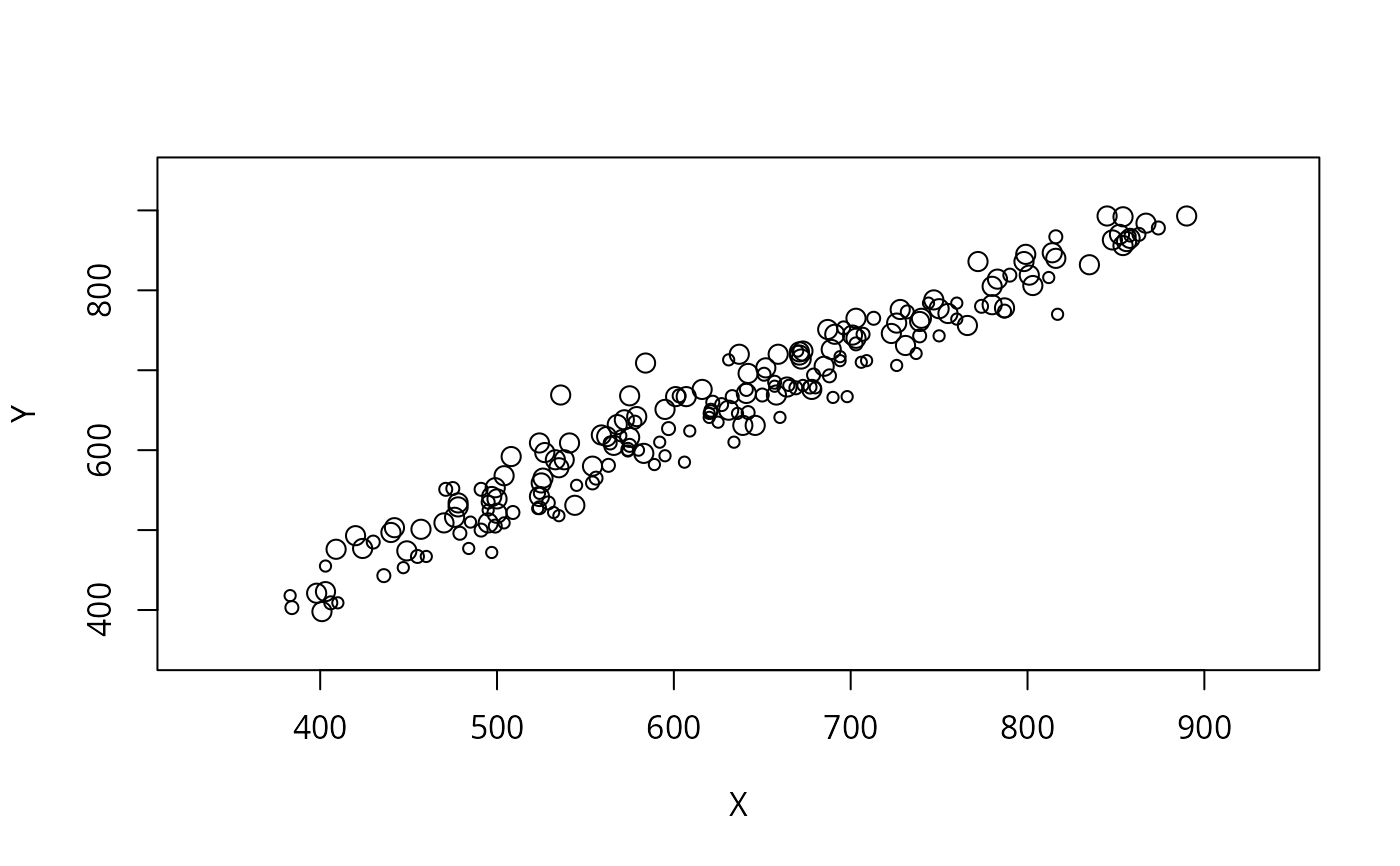
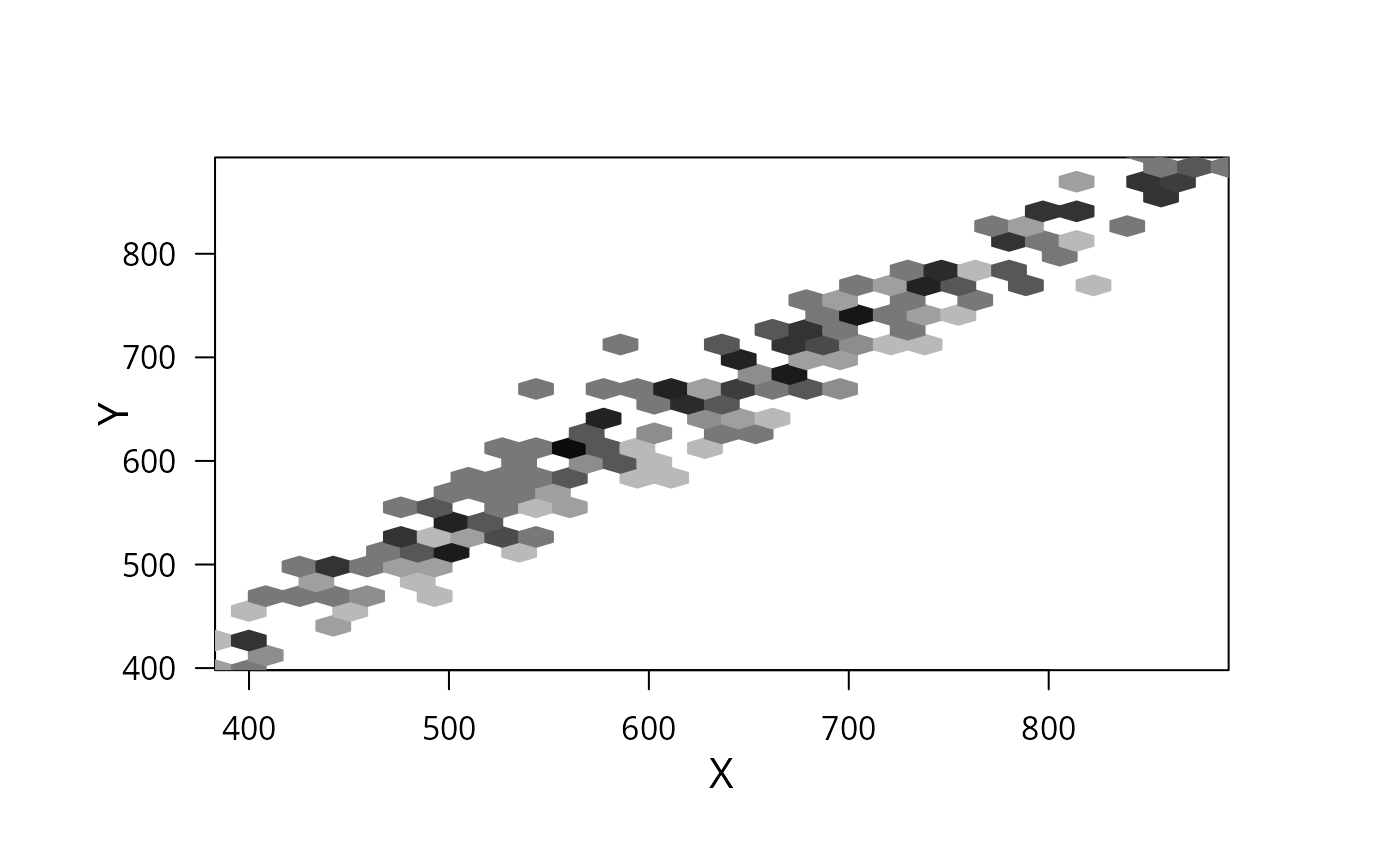
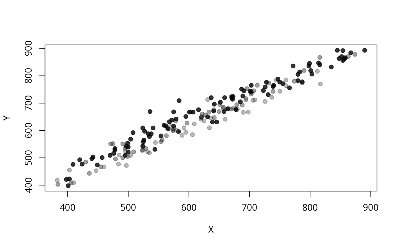
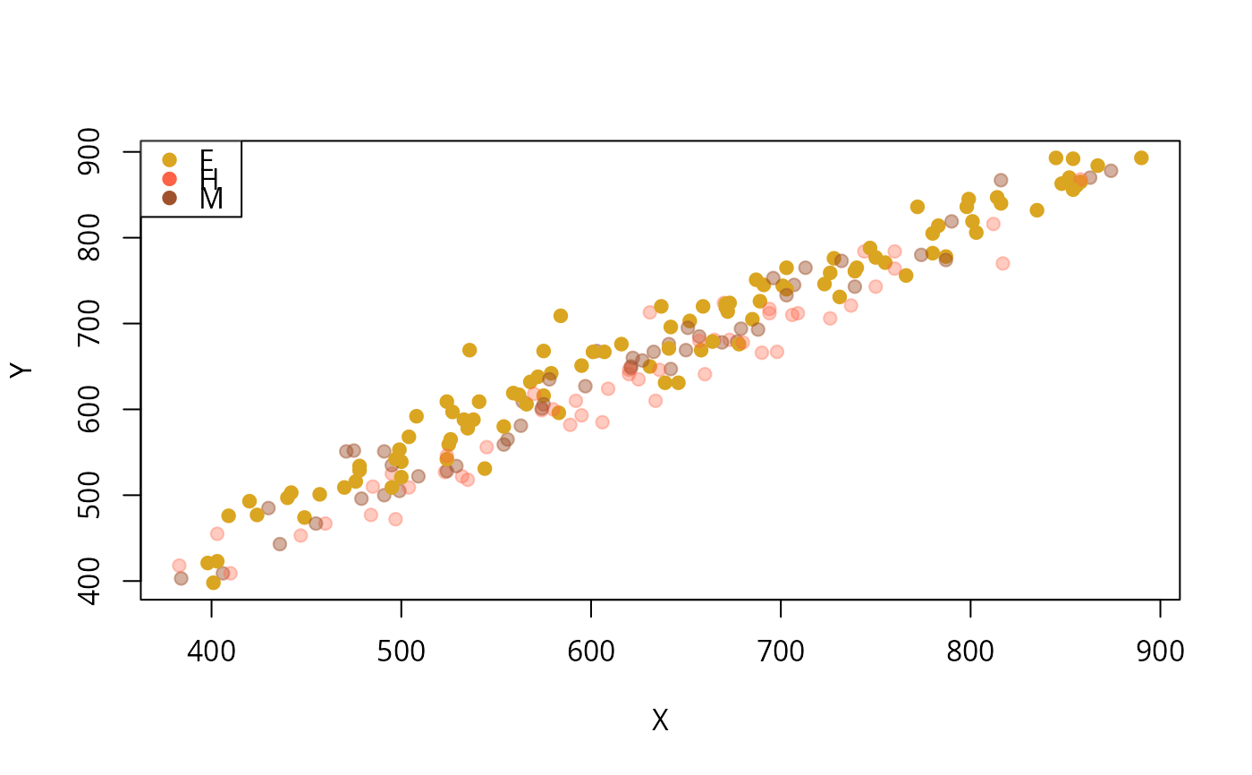
Bubble plots are scatterplots with circles whose area is proportional to the sampling weight. The two "hex" styles produce hexagonal binning scatterplots, and require the hexbin package from Bioconductor. The "transparent" style plots points with opacity proportional to sampling weight.

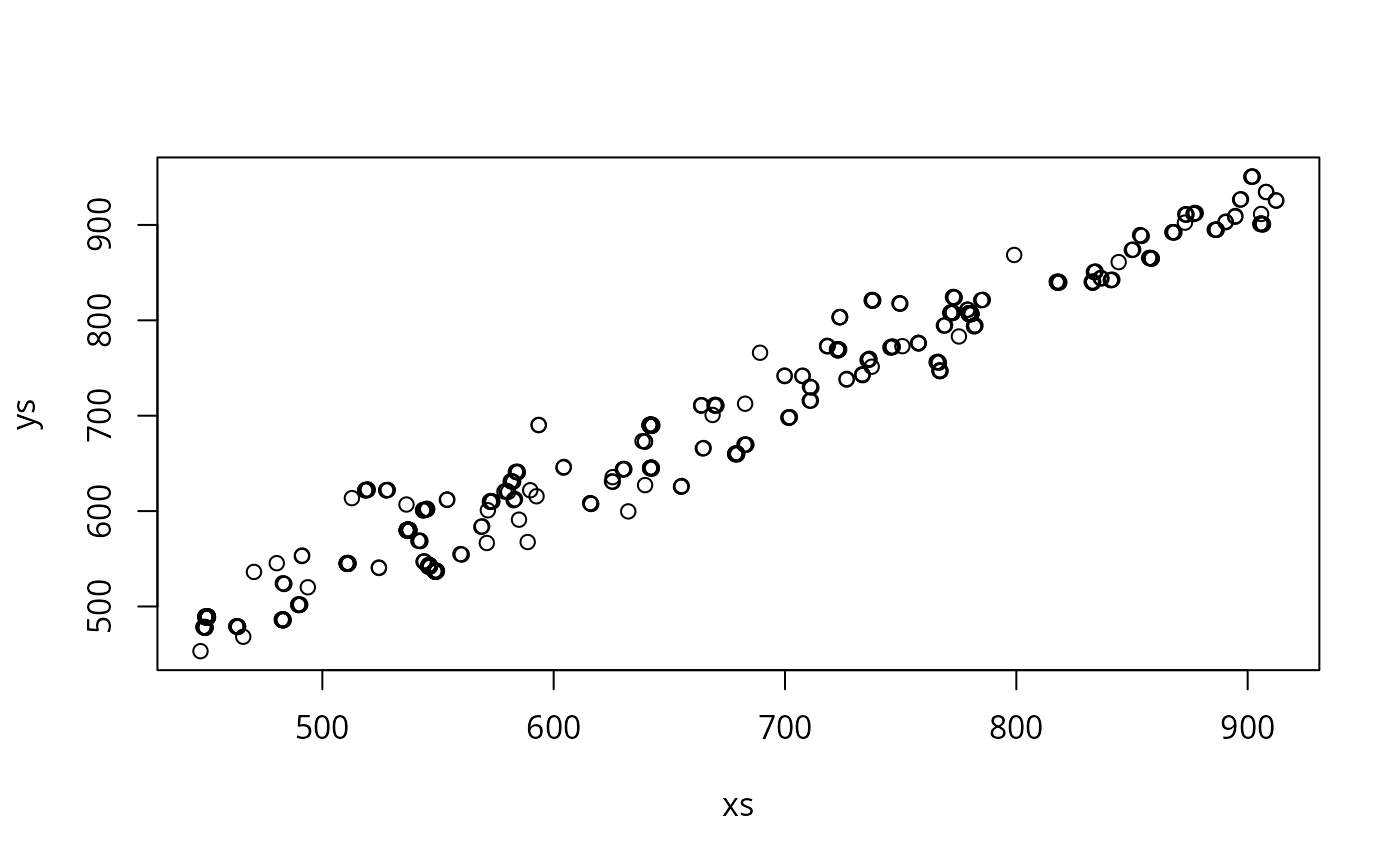
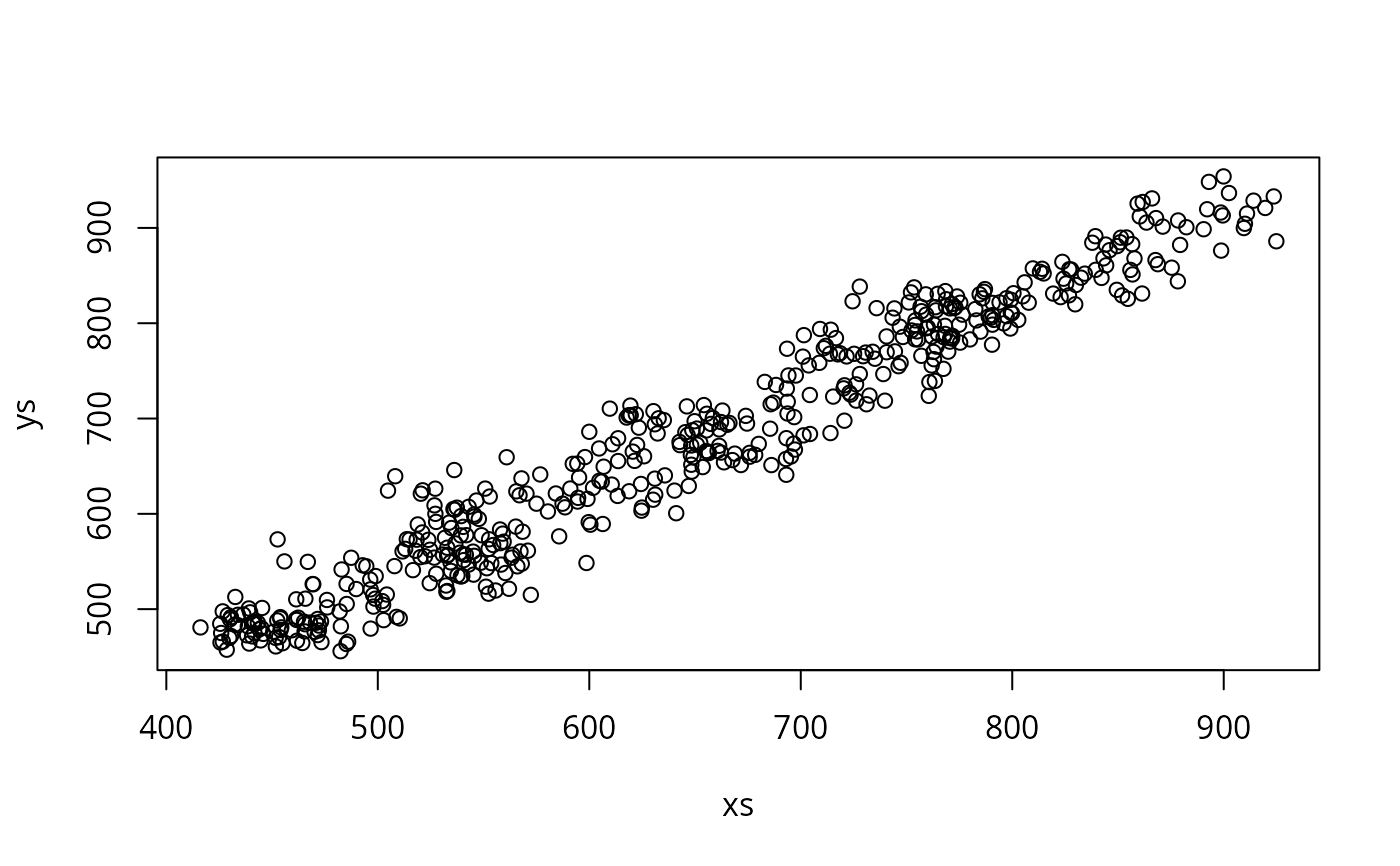
The subsample method uses the sampling weights to create a sample from approximately the population distribution and passes this to plot

Bubble plots are suited to small surveys, hexagonal binning and transparency to large surveys where plotting all the points would result in too much overlap.

basecol can be a function taking one data frame argument, which will be passed the data frame of variables from the survey object. This could be memory-intensive for large data sets.

Value

None

References

Korn EL, Graubard BI (1998) "Scatterplots with Survey Data" The American Statistician 52: 58-69

Lumley T, Scott A (2017) "Fitting Regression Models to Survey Data" Statistical Science 32: 265-278

Examples

data(api)
dstrat<-svydesign(id=~1,strata=~stype, weights=~pw, data=apistrat, fpc=~fpc)

svyplot(api00~api99, design=dstrat, style="bubble")

svyplot(api00~api99, design=dstrat, style="transparent",pch=19)


## these two require the hexbin package 
svyplot(api00~api99, design=dstrat, style="hex", xlab="1999 API",ylab="2000 API")

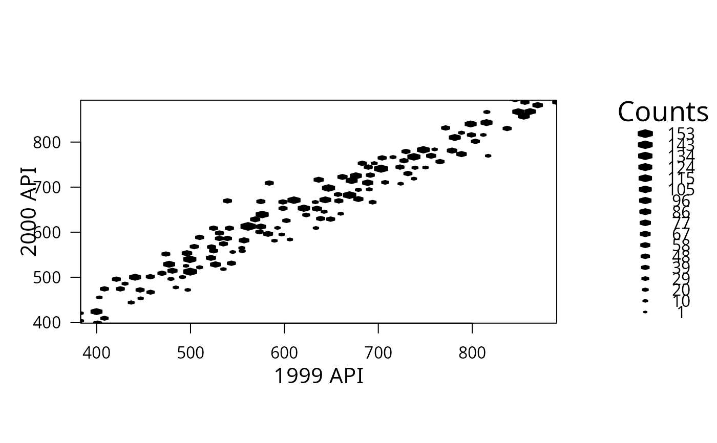svyplot(api00~api99, design=dstrat, style="grayhex",legend=0)



dclus2<-svydesign(id=~dnum+snum,  weights=~pw,
                    data=apiclus2, fpc=~fpc1+fpc2)
svyplot(api00~api99, design=dclus2, style="subsample")

svyplot(api00~api99, design=dclus2, style="subsample",
          amount=list(x=25,y=25))


svyplot(api00~api99, design=dstrat,
  basecol=function(df){c("goldenrod","tomato","sienna")[as.numeric(df$stype)]},
  style="transparent",pch=19,alpha=c(0,1))
legend("topleft",col=c("goldenrod","tomato","sienna"), pch=19, legend=c("E","H","M"))


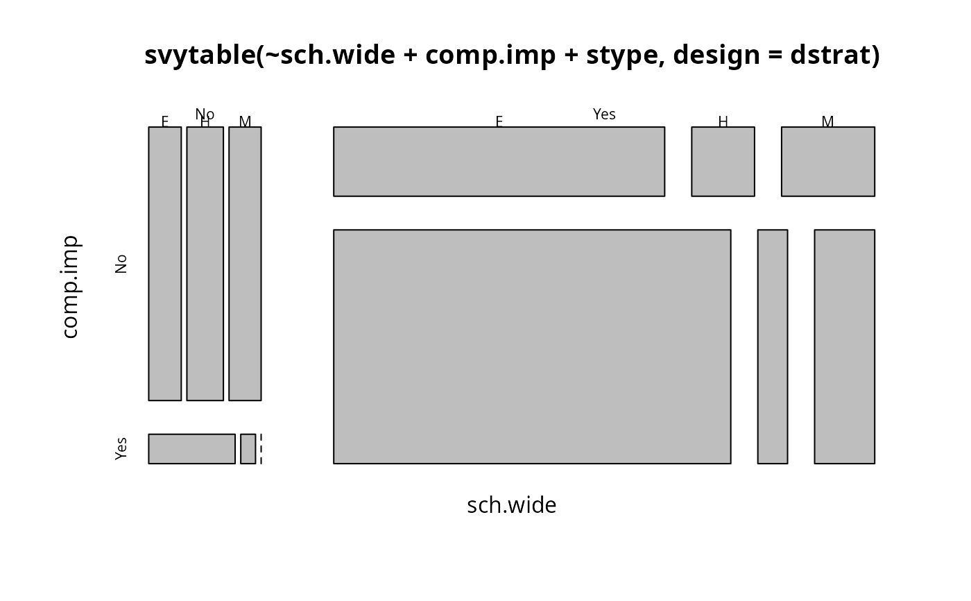
## For discrete data, estimate a population table and plot the table.
plot(svytable(~sch.wide+comp.imp+stype,design=dstrat))

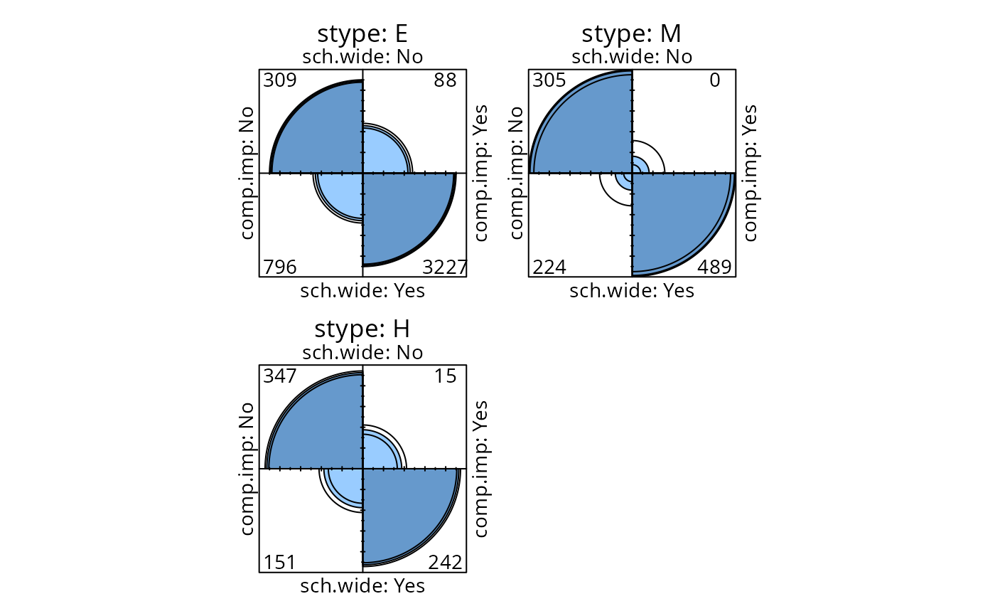
fourfoldplot(svytable(~sch.wide+comp.imp+stype,design=dstrat,round=TRUE))



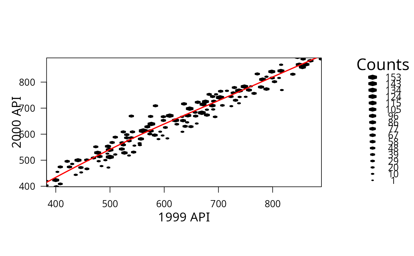
## To draw on a hexbin plot you need grid graphics, eg,
library(grid)
h<-svyplot(api00~api99, design=dstrat, style="hex", xlab="1999 API",ylab="2000 API")
s<-svysmooth(api00~api99,design=dstrat)
grid.polyline(s$api99$x,s$api99$y,vp=h$plot.vp@hexVp.on,default.units="native", 
   gp=gpar(col="red",lwd=2))