The Shrinkage t Statistic

shrinkt.stat and shrinkt.fun compute the “shrinkage t” statistic of Opgen-Rhein and Strimmer (2007).

Usage

shrinkt.stat(X, L, lambda.var, lambda.freqs, var.equal=TRUE, 
   paired=FALSE, verbose=TRUE)
shrinkt.fun(L, lambda.var, lambda.freqs, var.equal=TRUE, verbose=TRUE)

Arguments

X: data matrix. Note that the columns correspond to variables (“genes”) and the rows to samples.
L: factor with class labels for the two groups. If only a single label is given then a one-sample t-score against 0 is computed.
lambda.var: Shrinkage intensity for the variances. If not specified it is estimated from the data. lambda.var=0 implies no shrinkage and lambda.var=1 complete shrinkage.
lambda.freqs: Shrinkage intensity for the frequencies. If not specified it is estimated from the data. lambda.freqs=0 implies no shrinkage (i.e. empirical frequencies).
var.equal: assume equal (default) or unequal variances in each group.
paired: compute paired t-score (default is to use unpaired t-score).
verbose: print out some (more or less useful) information during computation.

Details

The “shrinkage t” statistic is similar to the usual t statistic, with the replacement of the sample variances by corresponding shrinkage estimates. These are derived in a distribution-free fashion and with little a priori assumptions. Using the “shrinkage t” statistic procduces highly accurate rankings - see Opgen-Rhein and Strimmer (2007).

The“shrinkage t” statistic can be generalized to include gene-wise correlation, see shrinkcat.stat.

The scale factor in the ”shrinkage t” statistic is computed from the estimated frequencies (to use the standard empirical scale factor set lambda.freqs=0).

Value

shrinkt.stat returns a vector containing the “shrinkage t” statistic for each variable/gene.

The corresponding shrinkt.fun functions return a function that produces the “shrinkage t” statistics when applied to a data matrix (this is very useful for simulations).

References

Opgen-Rhein, R., and K. Strimmer. 2007. Accurate ranking of differentially expressed genes by a distribution-free shrinkage approach. Statist. Appl. Genet. Mol. Biol. 6:9. <DOI:10.2202/1544-6115.1252>

Author

Rainer Opgen-Rhein, Verena Zuber, and Korbinian Strimmer (https://strimmerlab.github.io).

Examples

# load st library 
library("st")

# load Choe et al. (2005) data
data(choedata)
X <- choe2.mat
dim(X) # 6 11475  
#> [1]     6 11475
L <- choe2.L
L
#> [1] 1 1 1 2 2 2

# L may also contain some real labels
L = c("group 1", "group 1", "group 1", "group 2", "group 2", "group 2")

# shrinkage t statistic (equal variances)
score = shrinkt.stat(X, L)
#> Number of variables: 11475 
#> Number of observations: 6 
#> Number of classes: 2 
#> 
#> Estimating optimal shrinkage intensity lambda.freq (frequencies): 1 
#> Estimating variances (pooled across classes)
#> Estimating optimal shrinkage intensity lambda.var (variance vector): 0.3882 
#> 
order(score^2, decreasing=TRUE)[1:10]
#>  [1] 10979 11068    50  1022   724  5762    43  4790 10936  9939

# [1] 10979 11068    50  1022   724  5762    43  4790 10936  9939
#  lambda.var (variances):  0.3882
#  lambda.freqs (frequencies):  1

# shrinkage t statistic (unequal variances)
score = shrinkt.stat(X, L, var.equal=FALSE)
#> Number of variables: 11475 
#> Number of observations: 6 
#> Number of classes: 2 
#> 
#> Estimating optimal shrinkage intensity lambda.freq (frequencies): 1 
#> Estimating variances (class #1)
#> Estimating optimal shrinkage intensity lambda.var (variance vector): 0.3673 
#> 
#> Estimating variances (class #2)
#> Estimating optimal shrinkage intensity lambda.var (variance vector): 0.3362 
#> 
#> Estimating variances (pooled across classes)
#> Estimating optimal shrinkage intensity lambda.var (variance vector): 0.3882 
#> 
order(score^2, decreasing=TRUE)[1:10]
#>  [1] 11068    50 10979   724    43  1022  5762 10936  9939  9769

# [1] 11068    50 10979   724    43  1022  5762 10936  9939  9769
#  lambda.var class #1 and class #2 (variances):  0.3673   0.3362
#  lambda.freqs (frequencies): 1

# compute q-values and local false discovery rates
library("fdrtool")
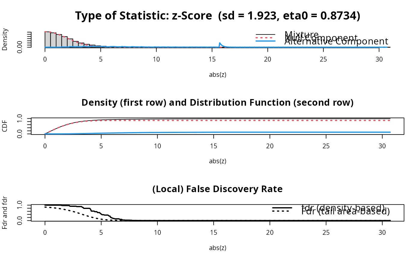
fdr.out = fdrtool(score) 
#> Step 1... determine cutoff point
#> Step 2... estimate parameters of null distribution and eta0
#> Step 3... compute p-values and estimate empirical PDF/CDF
#> Step 4... compute q-values and local fdr
#> Step 5... prepare for plotting

#> 
sum( fdr.out$qval < 0.05 )
#> [1] 894
sum( fdr.out$lfdr < 0.2 )
#> [1] 846
fdr.out$param
#>        cutoff N.cens     eta0    eta0.SE      sd     sd.SE
#> [1,] 1.158258   4541 0.873391 0.01007508 1.92272 0.2685543


# computation of paired t-score

# paired shrinkage t statistic
score = shrinkt.stat(X, L, paired=TRUE)
#> Number of variables: 11475 
#> Number of observations: 3 
#> Number of classes: 1 
#> 
#> Estimating optimal shrinkage intensity lambda.freq (frequencies): 1 
#> Estimating variances (pooled across classes)
#> Estimating optimal shrinkage intensity lambda.var (variance vector): 0.3498 
#> 
order(score^2, decreasing=TRUE)[1:10]
#>  [1]    50  4790  5393 11068  5762 10238  9939   708   728    68
# [1] 50  4790  5393 11068  5762 10238  9939   708   728    68


# if there is no shrinkage the paired shrinkage t score reduces
# to the conventional paired student t statistic
score = studentt.stat(X, L, paired=TRUE)
score2 = shrinkt.stat(X, L, lambda.var=0, lambda.freqs=0, paired=TRUE, verbose=FALSE)
sum((score-score2)^2)
#> [1] 0