Hazard Ratio Plot

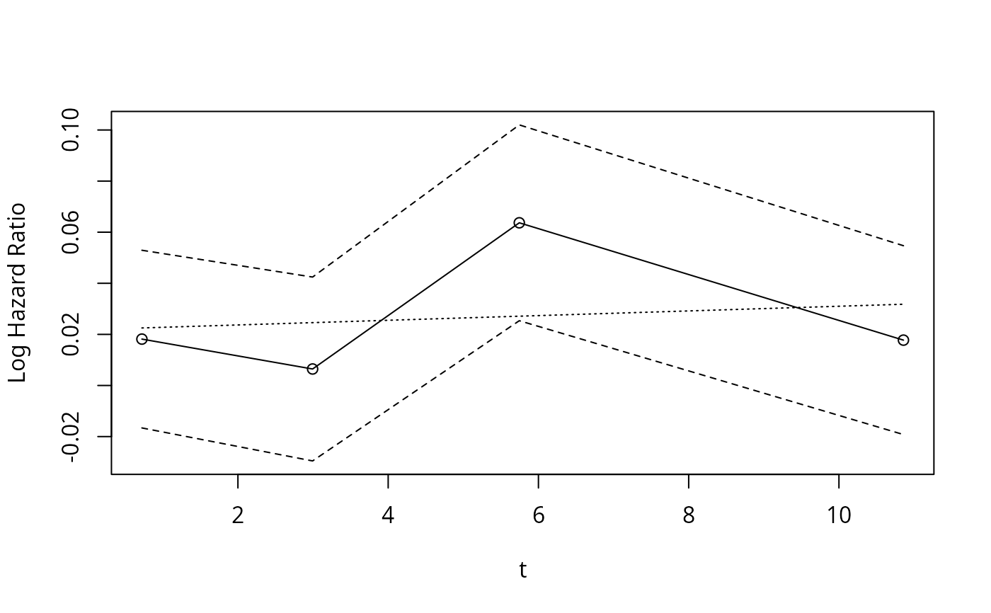
The hazard.ratio.plot function repeatedly estimates Cox regression coefficients and confidence limits within time intervals. The log hazard ratios are plotted against the mean failure/censoring time within the interval. Unless times is specified, the number of time intervals will be \(\max(round(d/e),2)\), where \(d\) is the total number of events in the sample. Efron's likelihood is used for estimating Cox regression coefficients (using coxph.fit). In the case of tied failure times, some intervals may have a point in common.

Usage

hazard.ratio.plot(x, Srv, which, times=, e=30, subset,
                  conf.int=.95, legendloc=NULL, smooth=TRUE, pr=FALSE, pl=TRUE,
                  add=FALSE, ylim, cex=.5, xlab="t", ylab, antilog=FALSE, ...)

Arguments

x

a vector or matrix of predictors

Srv

a Surv object

which

a vector of column numbers of x for which to estimate hazard ratios across time and make plots. The default is to do so for all predictors. Whenever one predictor is displayed, all other predictors in the x matrix are adjusted for (with a separate adjustment form for each time interval).

times

optional vector of time interval endpoints. Example: times=c(1,2,3) uses intervals [0,1), [1,2), [2,3), [3+). If times is omitted, uses intervals containing e events

e

number of events per time interval if times not given

subset

vector used for subsetting the entire analysis, e.g. subset=sex=="female"

conf.int

confidence interval coverage

legendloc

location for legend. Omit to use mouse, "none" for none, "ll" for lower left of graph, or actual x and y coordinates (e.g. c(2,3))

smooth

also plot the super–smoothed version of the log hazard ratios

pr

defaults to FALSE to suppress printing of individual Cox fits

pl

defaults to TRUE to plot results

add

add this plot to an already existing plot

ylim

vector of y-axis limits. Default is computed to include confidence bands.

cex

character size for legend information, default is 0.5

xlab

label for x-axis, default is "t"

ylab

label for y-axis, default is "Log Hazard Ratio" or "Hazard Ratio", depending on antilog.

antilog

default is FALSE. Set to TRUE to plot anti-log, i.e., hazard ratio.

...

optional graphical parameters

Author

Frank Harrell
Department of Biostatistics, Vanderbilt University
fh@fharrell.com

See also

cox.zph, residuals.cph, survival-internal, cph, coxph, Surv

Examples

require(survival)
n <- 500
set.seed(1)
age <- 50 + 12*rnorm(n)
cens <- 15*runif(n)
h <- .02*exp(.04*(age-50))
d.time <- -log(runif(n))/h
label(d.time) <- 'Follow-up Time'
e <- ifelse(d.time <= cens,1,0)
d.time <- pmin(d.time, cens)
units(d.time) <- "Year"
hazard.ratio.plot(age, Surv(d.time,e), e=20, legendloc='ll')

#> $time
#> [1]  0.72199  2.99413  5.74525 10.85871
#> 
#> $log.hazard.ratio
#>        [,1]      [,2]     [,3]     [,4]
#> x1 0.018155 0.0064516 0.063675 0.017749
#> 
#> $se
#>         [,1]    [,2]     [,3]     [,4]
#> [1,] 0.01774 0.01836 0.019553 0.018855
#>