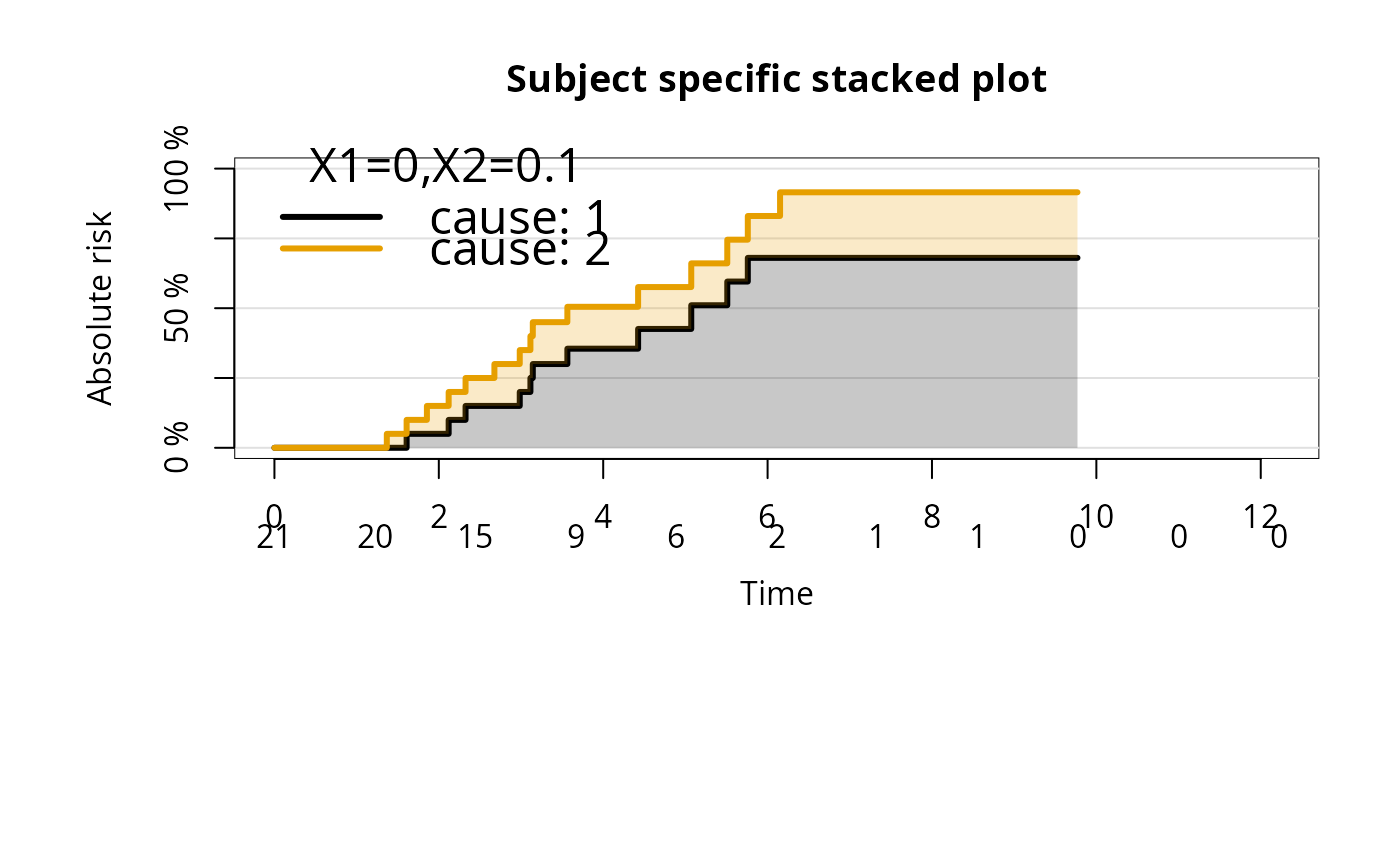
Function to plot survival probabilities or absolute risks (cumulative incidence function) against time.
Usage
# S3 method for class 'prodlim'
plot(
  x,
  type,
  cause,
  select,
  newdata,
  add = FALSE,
  col,
  lty,
  lwd,
  ylim,
  xlim,
  ylab,
  xlab = "Time",
  num.digits = 2,
  timeconverter,
  legend = TRUE,
  short.labels = TRUE,
  logrank = FALSE,
  marktime = FALSE,
  confint = TRUE,
  automar,
  atrisk = ifelse(add, FALSE, TRUE),
  timeOrigin = 0,
  axes = TRUE,
  background = TRUE,
  percent = TRUE,
  minAtrisk = 0,
  limit = 10,
  ...
)
Arguments
- x
an object of class `prodlim' as returned by the
prodlimfunction.- type
Either
"surv"or"risk"AKA"cuminc". Controls what part of the object is plotted. Defaults toobject$type.- cause
For competing risk models. Character (other classes are converted with
as.character). The argumentcausedetermines the event of interest. Currently one cause is allowed at a time, but you can call the function again withadd=TRUEto add the lines of the other causes. Also, ifcause="stacked"is specified the absolute risks of all causes are stacked.- select
Select which lines to plot. This can be used when there are many strata or many competing risks to select a subset of the lines. However, a more clean way to select covariate strata is to use the argument
newdata. Another application is when there are several competing risks and the stacked plot (cause="stacked") should only show a selected subset of the available causes.- newdata
a data frame containing covariate strata for which to show curves. When omitted element
Xof objectxis used.- add
if
TRUEcurves are added to an existing plot.- col
color for curves. Default is
1:number(curves)- lty
line type for curves. Default is 1.
- lwd
line width for all curves. Default is 3.
- ylim
limits of the y-axis
- xlim
limits of the x-axis
- ylab
label for the y-axis
- xlab
label for the x-axis
- num.digits
Number of digits when rounding off numerical values for legend and at-risk tables.
- timeconverter
The following options are supported: "days2years" (conversion factor: 1/365.25) "months2years" (conversion factor: 1/12) "days2months" (conversion factor 1/30.4368499) "years2days" (conversion factor 365.25) "years2months" (conversion factor 12) "months2days" (conversion factor 30.4368499)
- legend
if TRUE a legend is plotted by calling the function legend. Optional arguments of the function
legendcan be given in the formlegend.x=valwhere x is the name of the argument and val the desired value. See also Details.- short.labels
Logical. When
FALSEconstruct labels as cause=1, var1=v1, var2=v2 else as 1, v1, v2.- logrank
If TRUE, the logrank p-value will be extracted from a call to
survdiffand added to the legend. This works only for survival models, i.e. Kaplan-Meier with discrete predictors.- marktime
if TRUE the curves are tick-marked at right censoring times by invoking the function
markTime. Optional arguments of the functionmarkTimecan be given in the formconfint.x=valas with legend. See also Details.- confint
Logical. If
TRUEpointwise confidence intervals are plotted by invoking the functionconfInt. Optional arguments of the functionconfIntcan be given in the formconfint.x=valas with legend. See also Details.- automar
If TRUE the function trys to find suitable values for the figure margins around the main plotting region.
- atrisk
if TRUE display numbers of subjects at risk by invoking the function
atRisk. Optional arguments of the functionatRiskcan be given in the formatrisk.x=valas with legend. See also Details.- timeOrigin
Start of the time axis
- axes
If true axes are drawn. See details.
- background
If
TRUEthe background color and grid color can be controlled using smart arguments SmartControl, such as background.bg="yellow" or background.bg=c("gray66","gray88"). The following defaults are passed tobackgroundbyplot.prodlim: horizontal=seq(0,1,.25), vertical=NULL, bg="gray77", fg="white". Seebackgroundfor all arguments, and the examples below.- percent
If true the y-axis is labeled in percent.
- minAtrisk
Integer. Show the curve only until the number at-risk is at least
minAtrisk- limit
When newdata is not specified and the number of lines in element
Xof objectxexceeds limits, only the results for covariate constellations of the first, the middle and the last row inXare shown. Otherwise all lines ofXare shown.- ...
Parameters that are filtered by
SmartControland then passed to the functionsplot,legend,axis,atRisk,confInt,markTime,backGround
Details
From version 1.1.3 on the arguments legend.args, atrisk.args, confint.args
are obsolete and only available for backward compatibility. Instead
arguments for the invoked functions atRisk, legend,
confInt, markTime, axis are simply specified as
atrisk.cex=2. The specification is not case sensitive, thus
atRisk.cex=2 or atRISK.cex=2 will have the same effect. The
function axis is called twice, and arguments of the form
axis1.labels, axis1.at are used for the time axis whereas
axis2.pos, axis1.labels, etc. are used for the y-axis.
These arguments are processed via ...{} of plot.prodlim and
inside by using the function SmartControl. Documentation of these
arguments can be found in the help pages of the corresponding functions.
Examples
## simulate right censored data from a two state model
set.seed(100)
dat <- SimSurv(100)
# with(dat,plot(Hist(time,status)))
### marginal Kaplan-Meier estimator
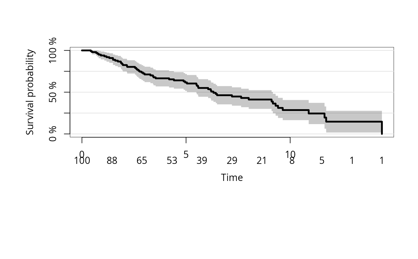
kmfit <- prodlim(Hist(time, status) ~ 1, data = dat)
plot(kmfit)
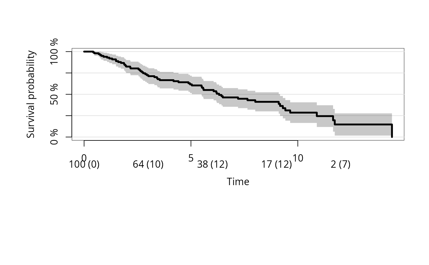
 plot(kmfit,atrisk.show.censored=1L,atrisk.at=seq(0,12,3))
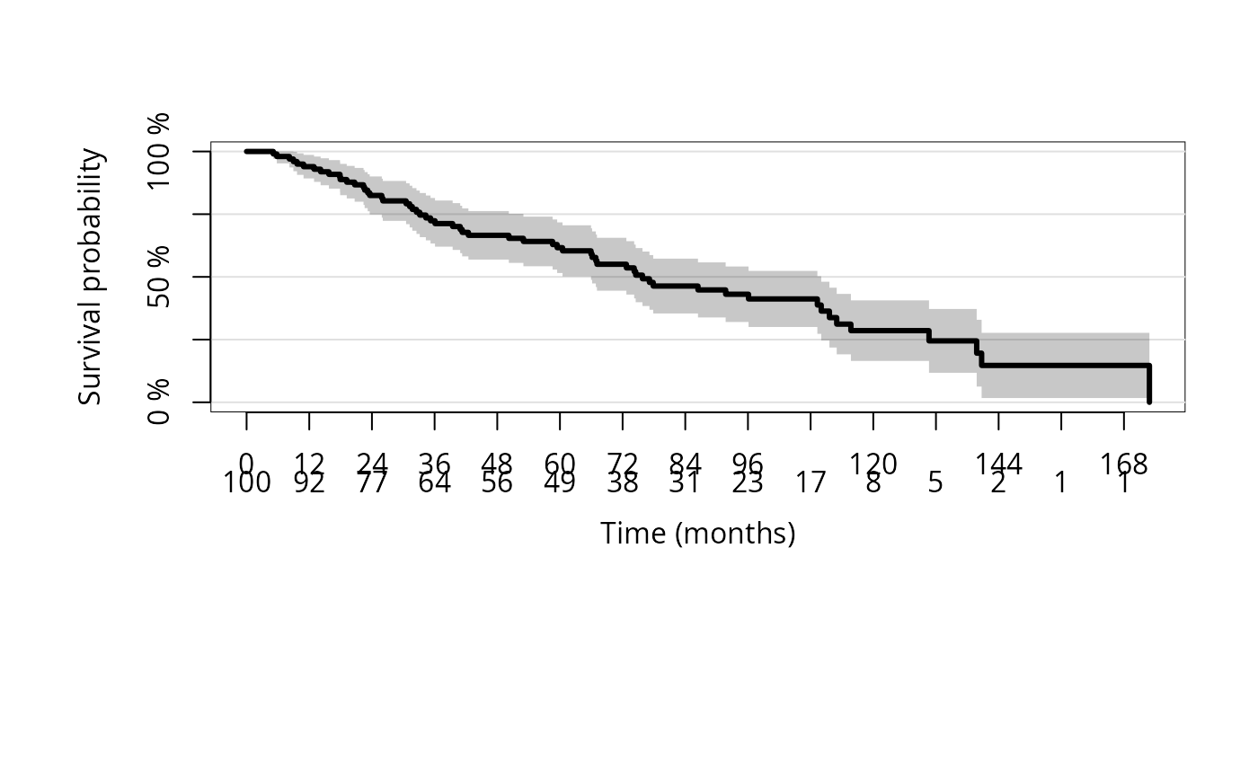
 plot(kmfit,timeconverter="years2months")
 # change time range
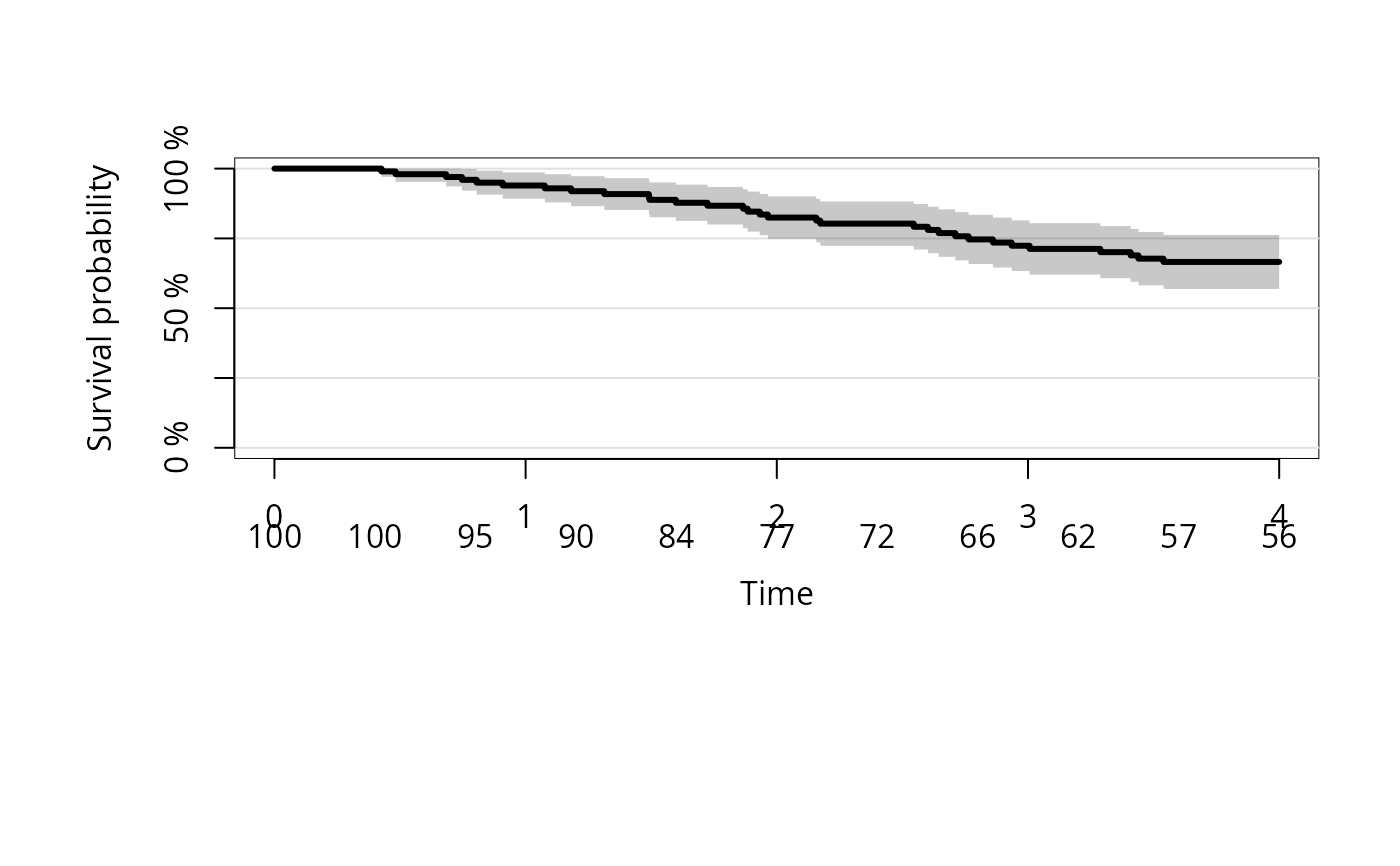
plot(kmfit,xlim=c(0,4))
# change time range
plot(kmfit,xlim=c(0,4))
 # change scale of y-axis
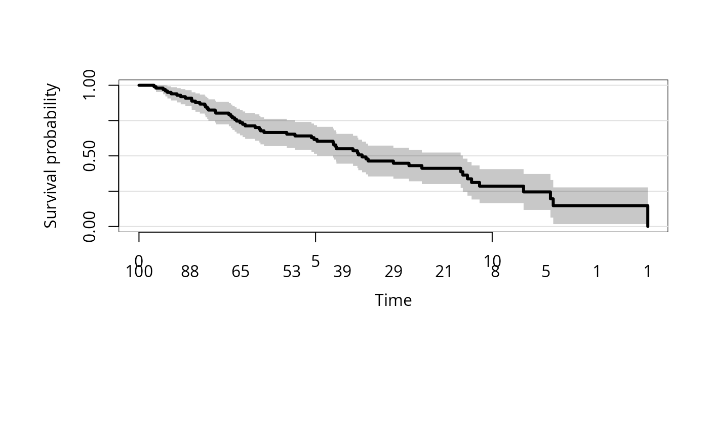
plot(kmfit,percent=FALSE)
# change scale of y-axis
plot(kmfit,percent=FALSE)
 # mortality instead of survival
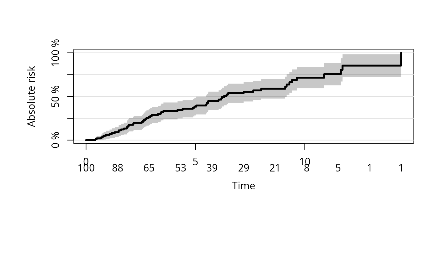
plot(kmfit,type="risk")
# mortality instead of survival
plot(kmfit,type="risk")
 # change axis label and position of ticks
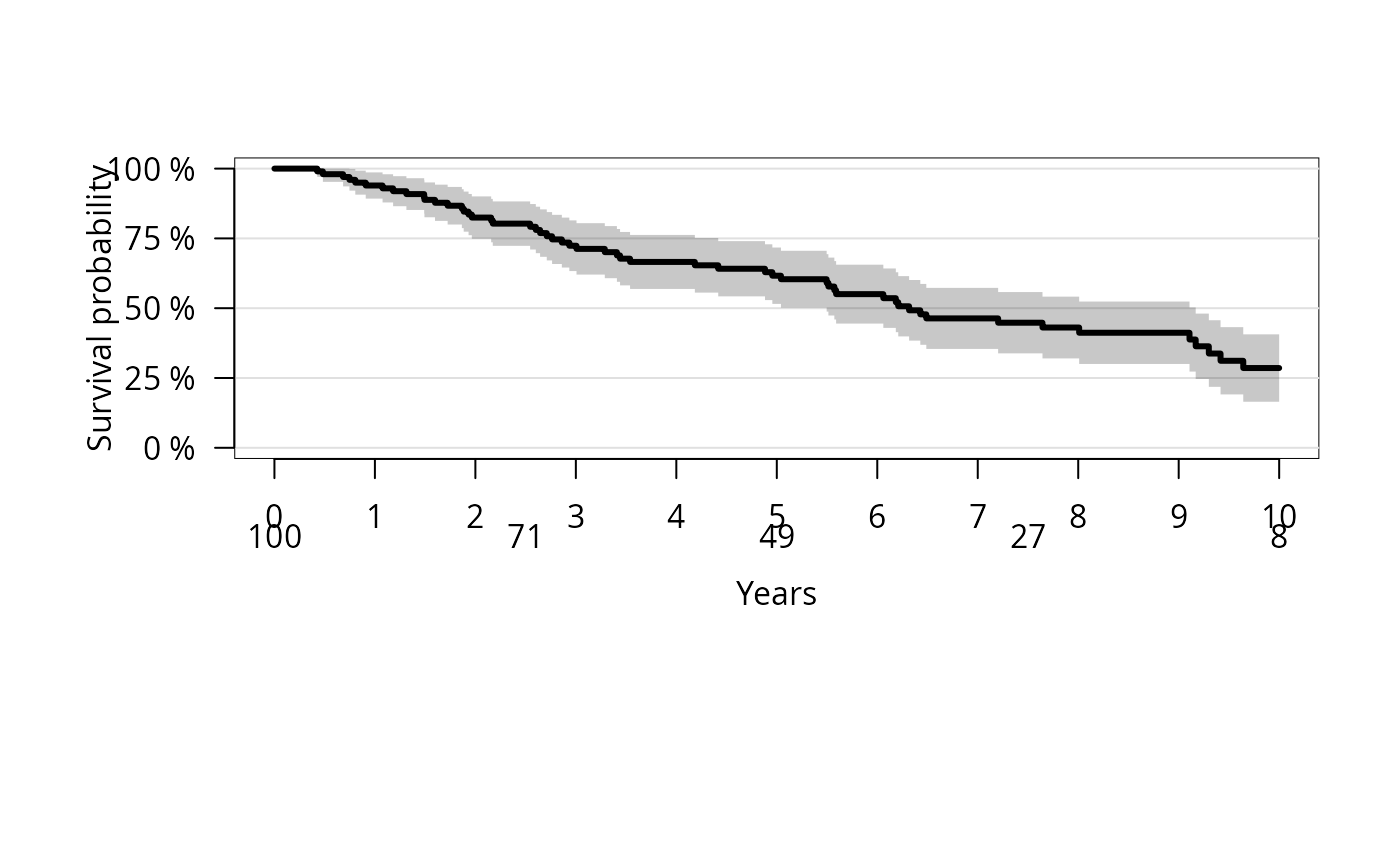
plot(kmfit,
xlim=c(0,10),
axis1.at=seq(0,10,1),
axis1.labels=0:10,
xlab="Years",
axis2.las=2,
atrisk.at=seq(0,10,2.5),
atrisk.title="")
# change axis label and position of ticks
plot(kmfit,
xlim=c(0,10),
axis1.at=seq(0,10,1),
axis1.labels=0:10,
xlab="Years",
axis2.las=2,
atrisk.at=seq(0,10,2.5),
atrisk.title="")
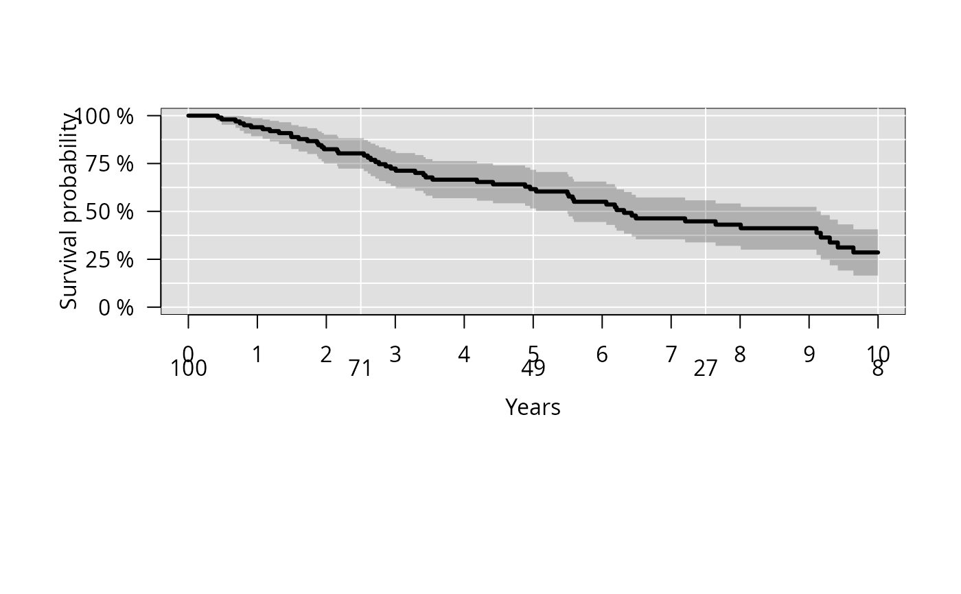
 # change background color
plot(kmfit,
xlim=c(0,10),
confint.citype="shadow",
col=1,
axis1.at=0:10,
axis1.labels=0:10,
xlab="Years",
axis2.las=2,
atrisk.at=seq(0,10,2.5),
atrisk.title="",
background=TRUE,
background.fg="white",
background.horizontal=seq(0,1,.25/2),
background.vertical=seq(0,10,2.5),
background.bg=c("gray88"))
# change background color
plot(kmfit,
xlim=c(0,10),
confint.citype="shadow",
col=1,
axis1.at=0:10,
axis1.labels=0:10,
xlab="Years",
axis2.las=2,
atrisk.at=seq(0,10,2.5),
atrisk.title="",
background=TRUE,
background.fg="white",
background.horizontal=seq(0,1,.25/2),
background.vertical=seq(0,10,2.5),
background.bg=c("gray88"))
 # change type of confidence limits
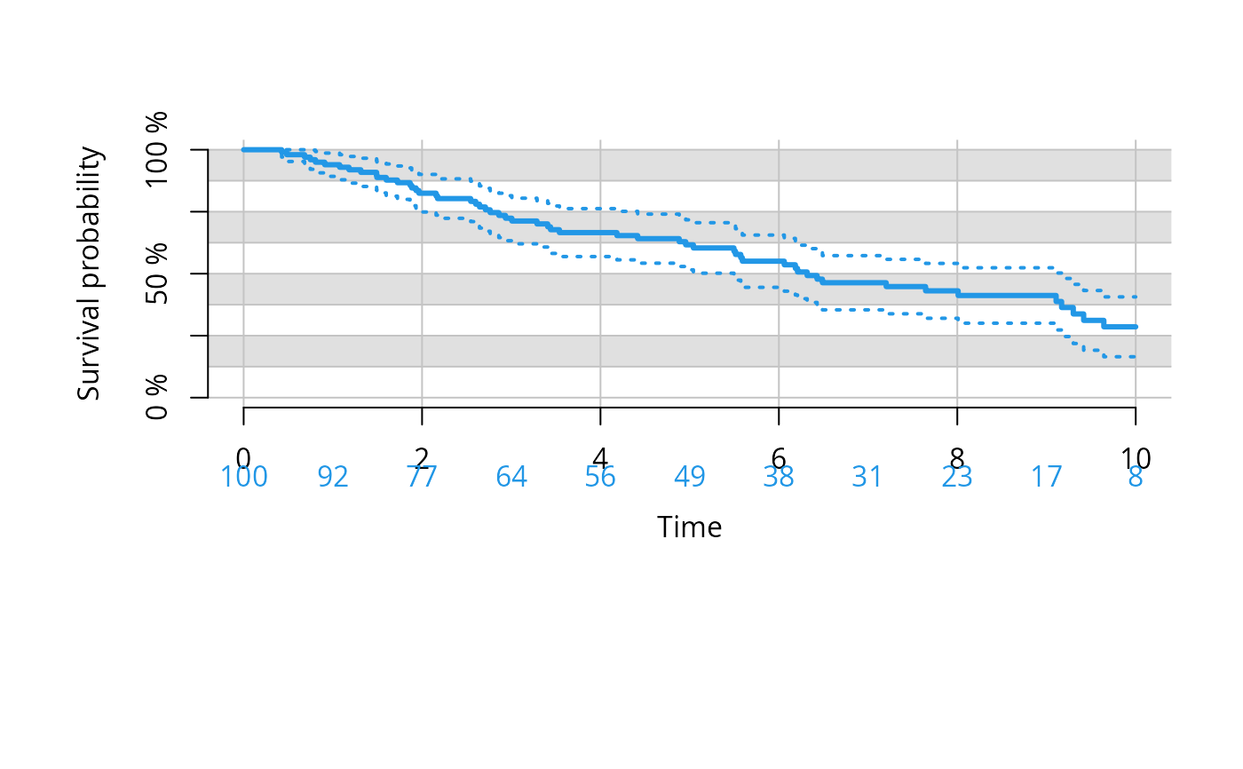
plot(kmfit,
xlim=c(0,10),
confint.citype="dots",
col=4,
background=TRUE,
background.bg=c("white","gray88"),
background.fg="gray77",
background.horizontal=seq(0,1,.25/2),
background.vertical=seq(0,10,2))
# change type of confidence limits
plot(kmfit,
xlim=c(0,10),
confint.citype="dots",
col=4,
background=TRUE,
background.bg=c("white","gray88"),
background.fg="gray77",
background.horizontal=seq(0,1,.25/2),
background.vertical=seq(0,10,2))
 ### Kaplan-Meier in discrete strata
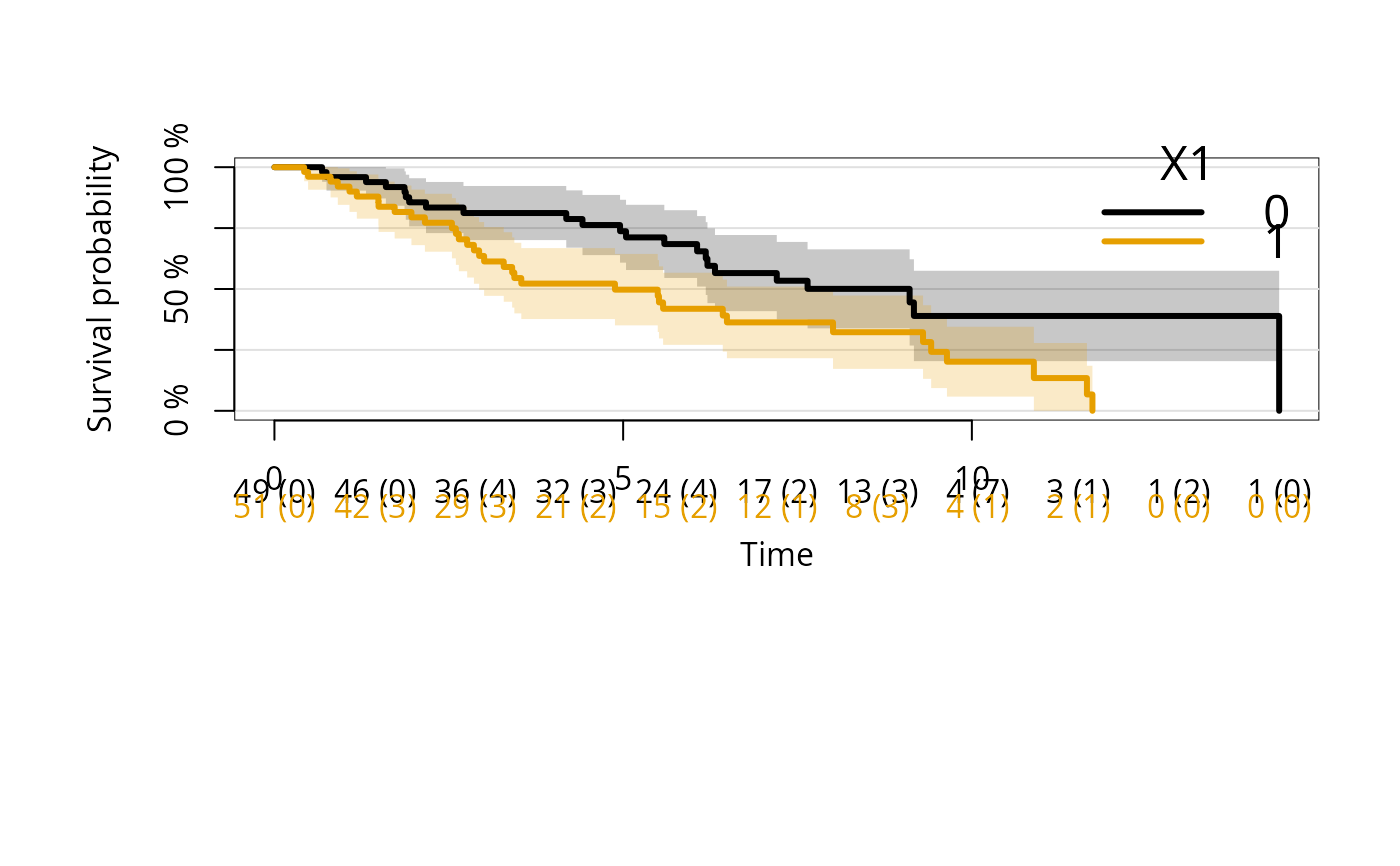
kmfitX <- prodlim(Hist(time, status) ~ X1, data = dat)
plot(kmfitX,atrisk.show.censored=1L)
### Kaplan-Meier in discrete strata
kmfitX <- prodlim(Hist(time, status) ~ X1, data = dat)
plot(kmfitX,atrisk.show.censored=1L)
 # move legend
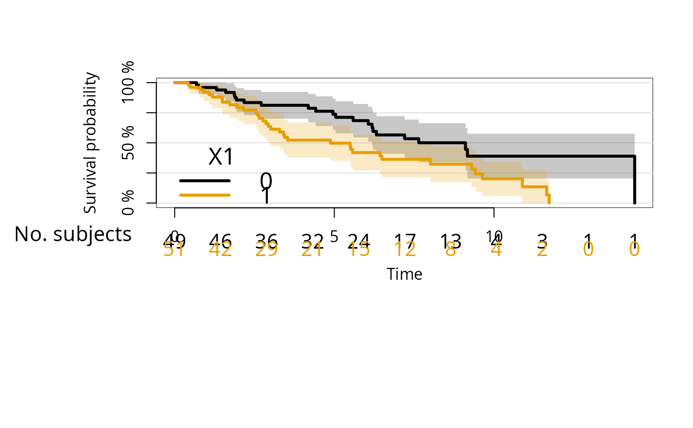
plot(kmfitX,legend.x="bottomleft",atRisk.cex=1.3,
atrisk.title="No. subjects")
# move legend
plot(kmfitX,legend.x="bottomleft",atRisk.cex=1.3,
atrisk.title="No. subjects")
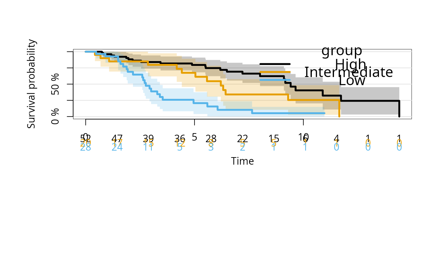
 ## Control the order of strata
## since version 1.5.1 prodlim does obey the order of
## factor levels
dat$group <- factor(cut(dat$X2,c(-Inf,0,0.5,Inf)),
labels=c("High","Intermediate","Low"))
kmfitG <- prodlim(Hist(time, status) ~ group, data = dat)
plot(kmfitG)
## Control the order of strata
## since version 1.5.1 prodlim does obey the order of
## factor levels
dat$group <- factor(cut(dat$X2,c(-Inf,0,0.5,Inf)),
labels=c("High","Intermediate","Low"))
kmfitG <- prodlim(Hist(time, status) ~ group, data = dat)
plot(kmfitG)
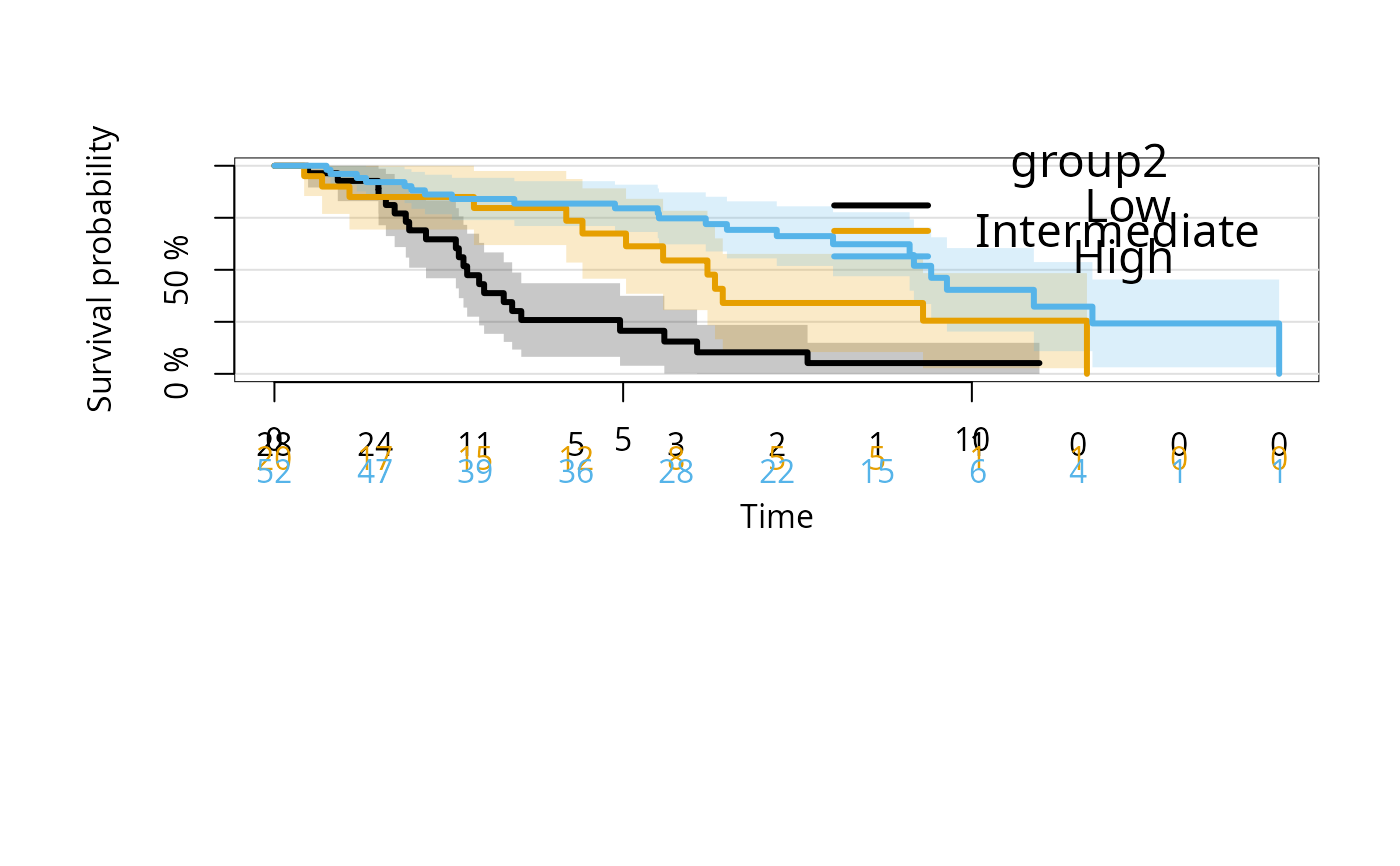
 ## relevel
dat$group2 <- factor(cut(dat$X2,c(-Inf,0,0.5,Inf)),
levels=c("(0.5, Inf]","(0,0.5]","(-Inf,0]"),
labels=c("Low","Intermediate","High"))
kmfitG2 <- prodlim(Hist(time, status) ~ group2, data = dat)
plot(kmfitG2)
## relevel
dat$group2 <- factor(cut(dat$X2,c(-Inf,0,0.5,Inf)),
levels=c("(0.5, Inf]","(0,0.5]","(-Inf,0]"),
labels=c("Low","Intermediate","High"))
kmfitG2 <- prodlim(Hist(time, status) ~ group2, data = dat)
plot(kmfitG2)
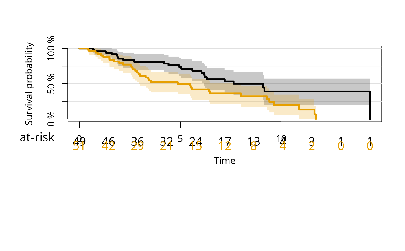
 # add log-rank test to legend
plot(kmfitX,
atRisk.cex=1.3,
logrank=TRUE,
legend.x="topright",
atrisk.title="at-risk")
# add log-rank test to legend
plot(kmfitX,
atRisk.cex=1.3,
logrank=TRUE,
legend.x="topright",
atrisk.title="at-risk")
 #> Error in eval(x$call$data): object 'dat' not found
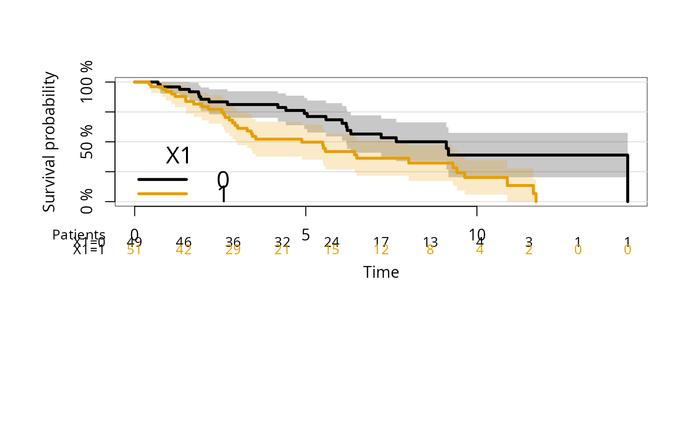
# change atrisk labels
plot(kmfitX,
legend.x="bottomleft",
atrisk.title="Patients",
atrisk.cex=0.9,
atrisk.labels=c("X1=0","X1=1"))
#> Error in eval(x$call$data): object 'dat' not found
# change atrisk labels
plot(kmfitX,
legend.x="bottomleft",
atrisk.title="Patients",
atrisk.cex=0.9,
atrisk.labels=c("X1=0","X1=1"))
 # multiple categorical factors
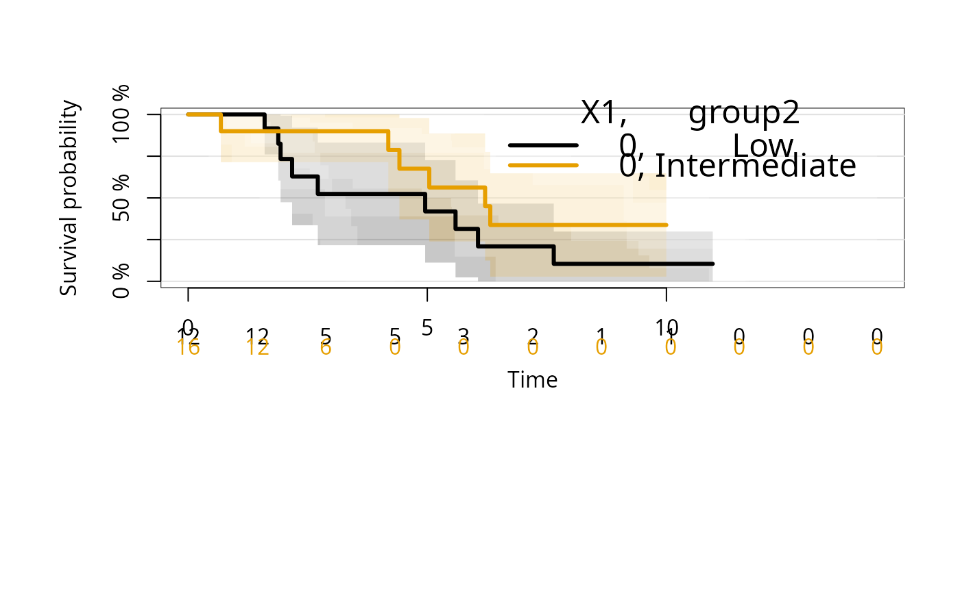
kmfitXG <- prodlim(Hist(time,status)~X1+group2,data=dat)
plot(kmfitXG,select=1:2)
# multiple categorical factors
kmfitXG <- prodlim(Hist(time,status)~X1+group2,data=dat)
plot(kmfitXG,select=1:2)
 ### Kaplan-Meier in continuous strata
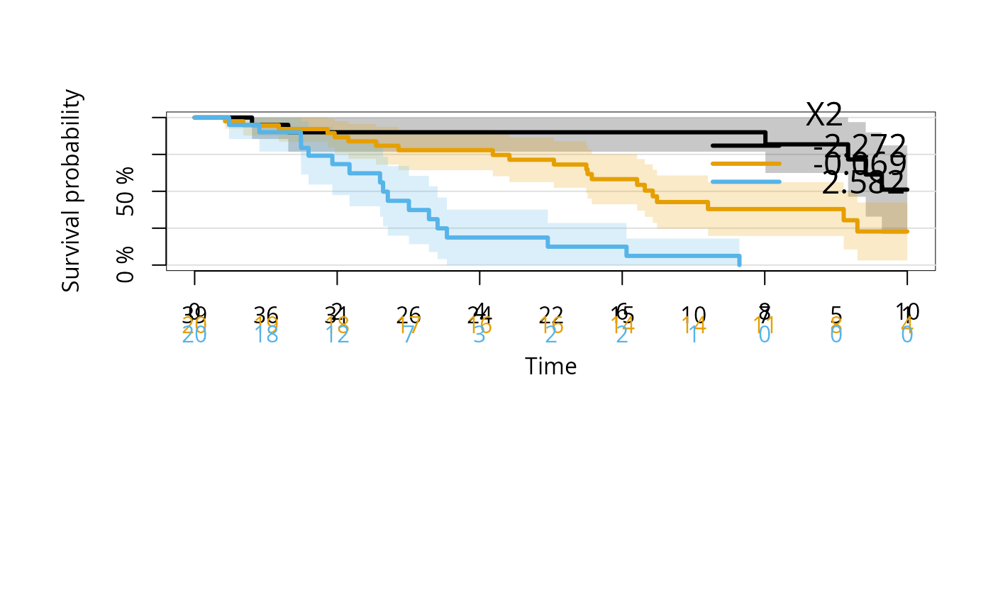
kmfitX2 <- prodlim(Hist(time, status) ~ X2, data = dat)
plot(kmfitX2,xlim=c(0,10))
### Kaplan-Meier in continuous strata
kmfitX2 <- prodlim(Hist(time, status) ~ X2, data = dat)
plot(kmfitX2,xlim=c(0,10))
 # specify values of X2 for which to show the curves
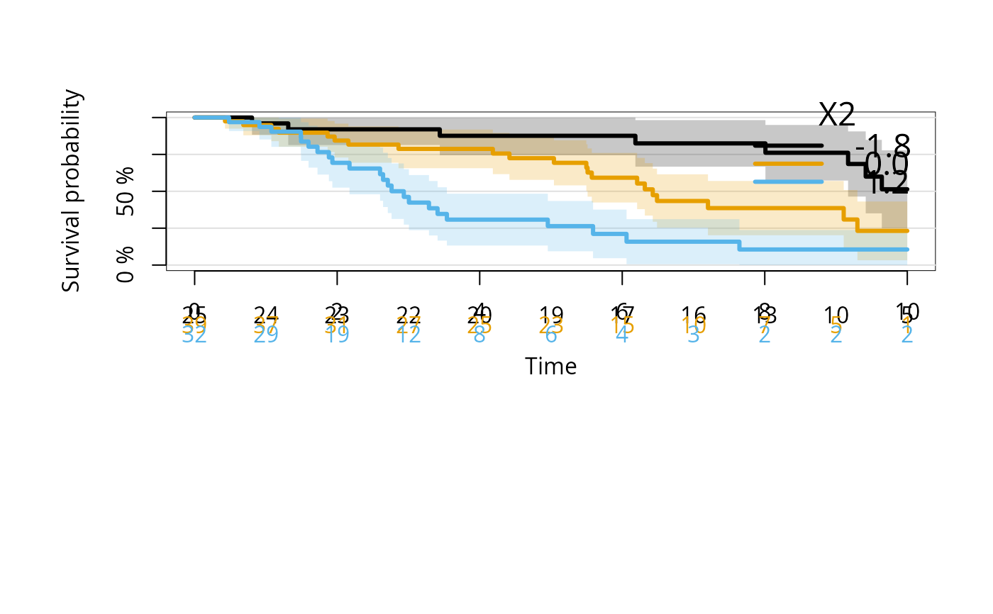
plot(kmfitX2,xlim=c(0,10),newdata=data.frame(X2=c(-1.8,0,1.2)))
# specify values of X2 for which to show the curves
plot(kmfitX2,xlim=c(0,10),newdata=data.frame(X2=c(-1.8,0,1.2)))
 ### Cluster-correlated data
library(survival)
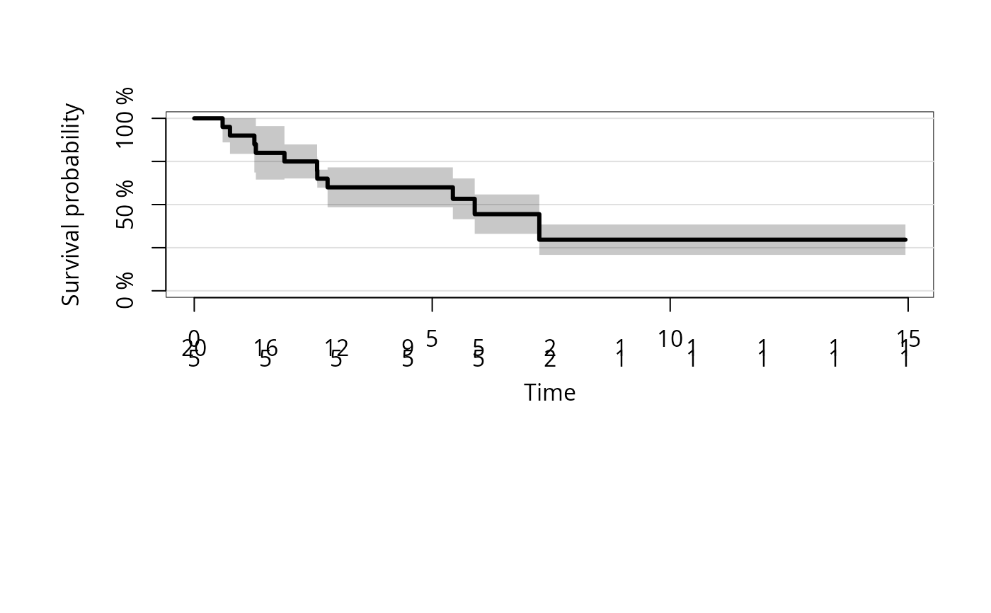
cdat <- cbind(SimSurv(20),patnr=sample(1:5,size=20,replace=TRUE))
kmfitC <- prodlim(Hist(time, status) ~ cluster(patnr), data = cdat)
plot(kmfitC)
### Cluster-correlated data
library(survival)
cdat <- cbind(SimSurv(20),patnr=sample(1:5,size=20,replace=TRUE))
kmfitC <- prodlim(Hist(time, status) ~ cluster(patnr), data = cdat)
plot(kmfitC)
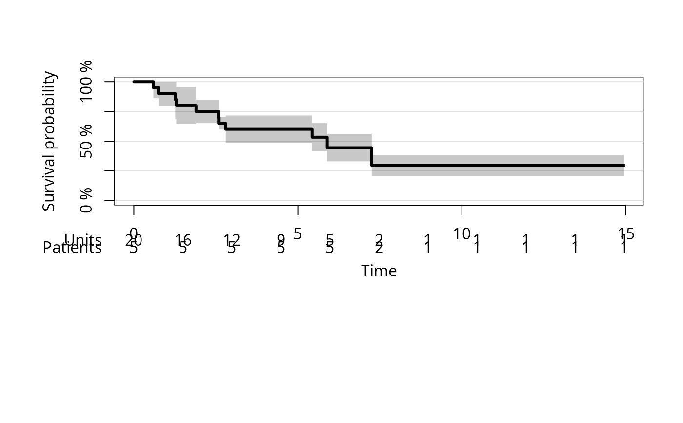
 plot(kmfitC,atrisk.labels=c("Units","Patients"))
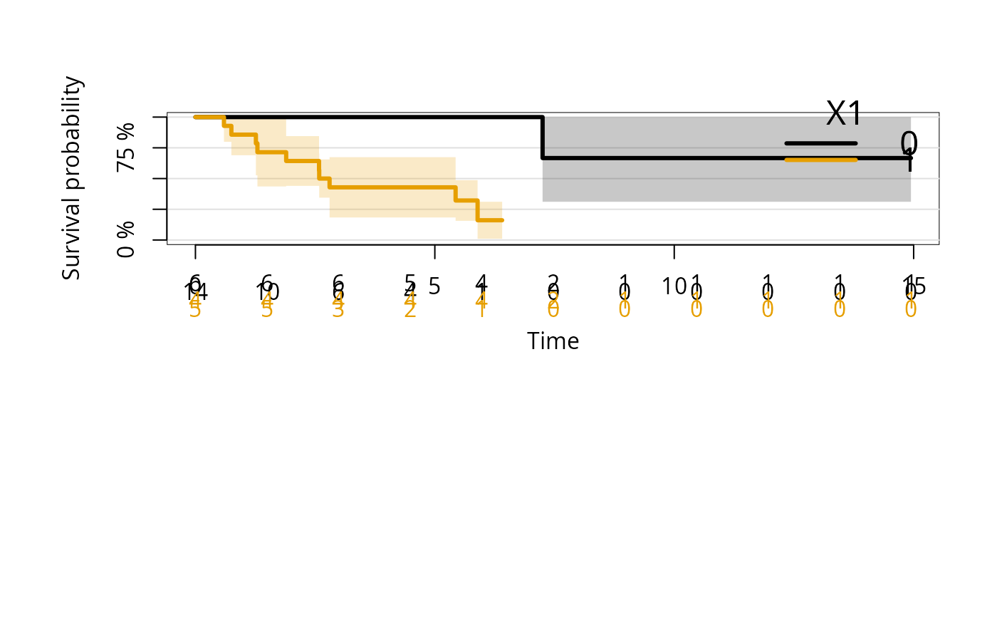
 kmfitC2 <- prodlim(Hist(time, status) ~ X1+cluster(patnr), data = cdat)
plot(kmfitC2)
kmfitC2 <- prodlim(Hist(time, status) ~ X1+cluster(patnr), data = cdat)
plot(kmfitC2)
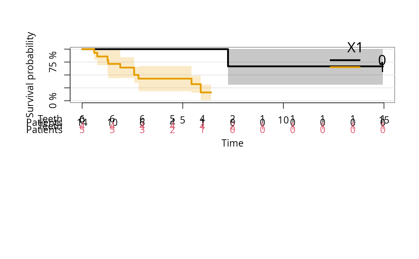
 plot(kmfitC2,atrisk.labels=c("Teeth","Patients","Teeth","Patients"),
atrisk.col=c(1,1,2,2))
plot(kmfitC2,atrisk.labels=c("Teeth","Patients","Teeth","Patients"),
atrisk.col=c(1,1,2,2))
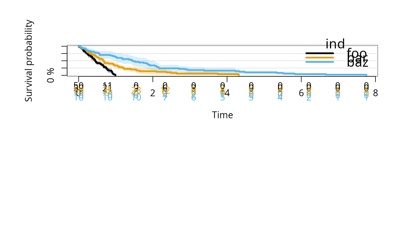
 ### Cluster-correlated data with strata
n = 50
foo = runif(n)
bar = rexp(n)
baz = rexp(n,1/2)
d = stack(data.frame(foo,bar,baz))
d$cl = sample(10, 3*n, replace=TRUE)
fit = prodlim(Surv(values) ~ ind + cluster(cl), data=d)
plot(fit)
### Cluster-correlated data with strata
n = 50
foo = runif(n)
bar = rexp(n)
baz = rexp(n,1/2)
d = stack(data.frame(foo,bar,baz))
d$cl = sample(10, 3*n, replace=TRUE)
fit = prodlim(Surv(values) ~ ind + cluster(cl), data=d)
plot(fit)
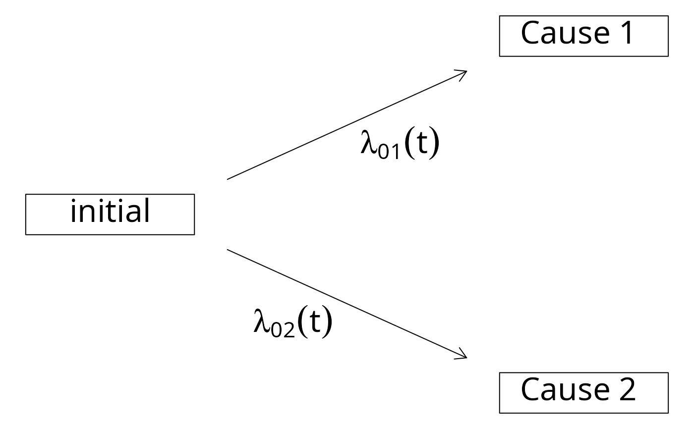
 ## simulate right censored data from a competing risk model
datCR <- SimCompRisk(100)
with(datCR,plot(Hist(time,event)))
#> Warning: The dimension of the boxes may depend on the current graphical device
#> in the sense that the layout and centering of text may change when you resize the graphical device and call the same plot.
## simulate right censored data from a competing risk model
datCR <- SimCompRisk(100)
with(datCR,plot(Hist(time,event)))
#> Warning: The dimension of the boxes may depend on the current graphical device
#> in the sense that the layout and centering of text may change when you resize the graphical device and call the same plot.
 ### marginal Aalen-Johansen estimator
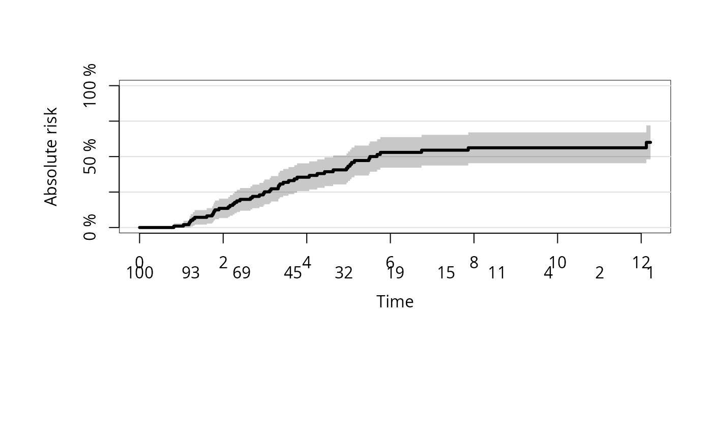
ajfit <- prodlim(Hist(time, event) ~ 1, data = datCR)
plot(ajfit) # same as plot(ajfit,cause=1)
### marginal Aalen-Johansen estimator
ajfit <- prodlim(Hist(time, event) ~ 1, data = datCR)
plot(ajfit) # same as plot(ajfit,cause=1)
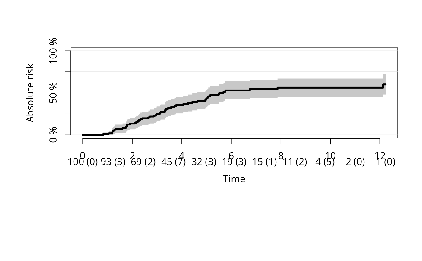
 plot(ajfit,atrisk.show.censored=1L)
 # cause 2
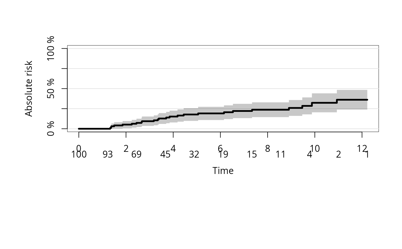
plot(ajfit,cause=2)
# cause 2
plot(ajfit,cause=2)
 # both in one
plot(ajfit,cause=1)
plot(ajfit,cause=2,add=TRUE,col=2)
# both in one
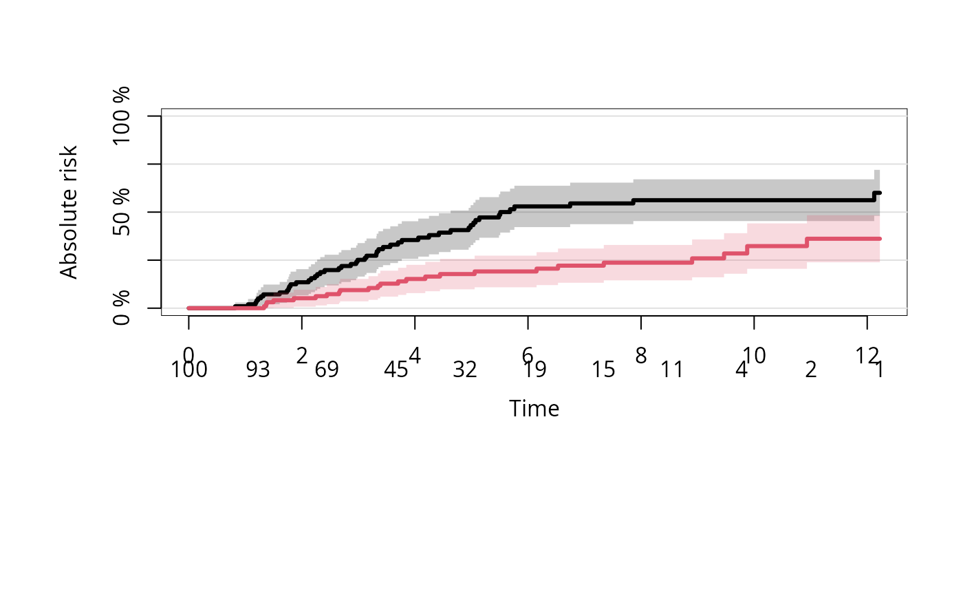
plot(ajfit,cause=1)
plot(ajfit,cause=2,add=TRUE,col=2)
 ### stacked plot
plot(ajfit,cause="stacked",select=2)
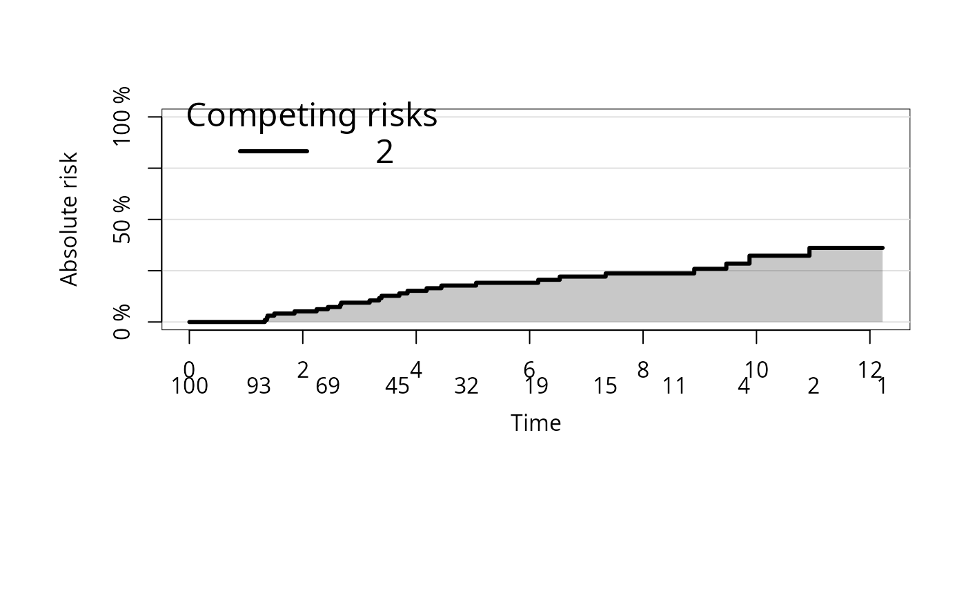
### stacked plot
plot(ajfit,cause="stacked",select=2)
 ### stratified Aalen-Johansen estimator
ajfitX1 <- prodlim(Hist(time, event) ~ X1, data = datCR)
plot(ajfitX1)
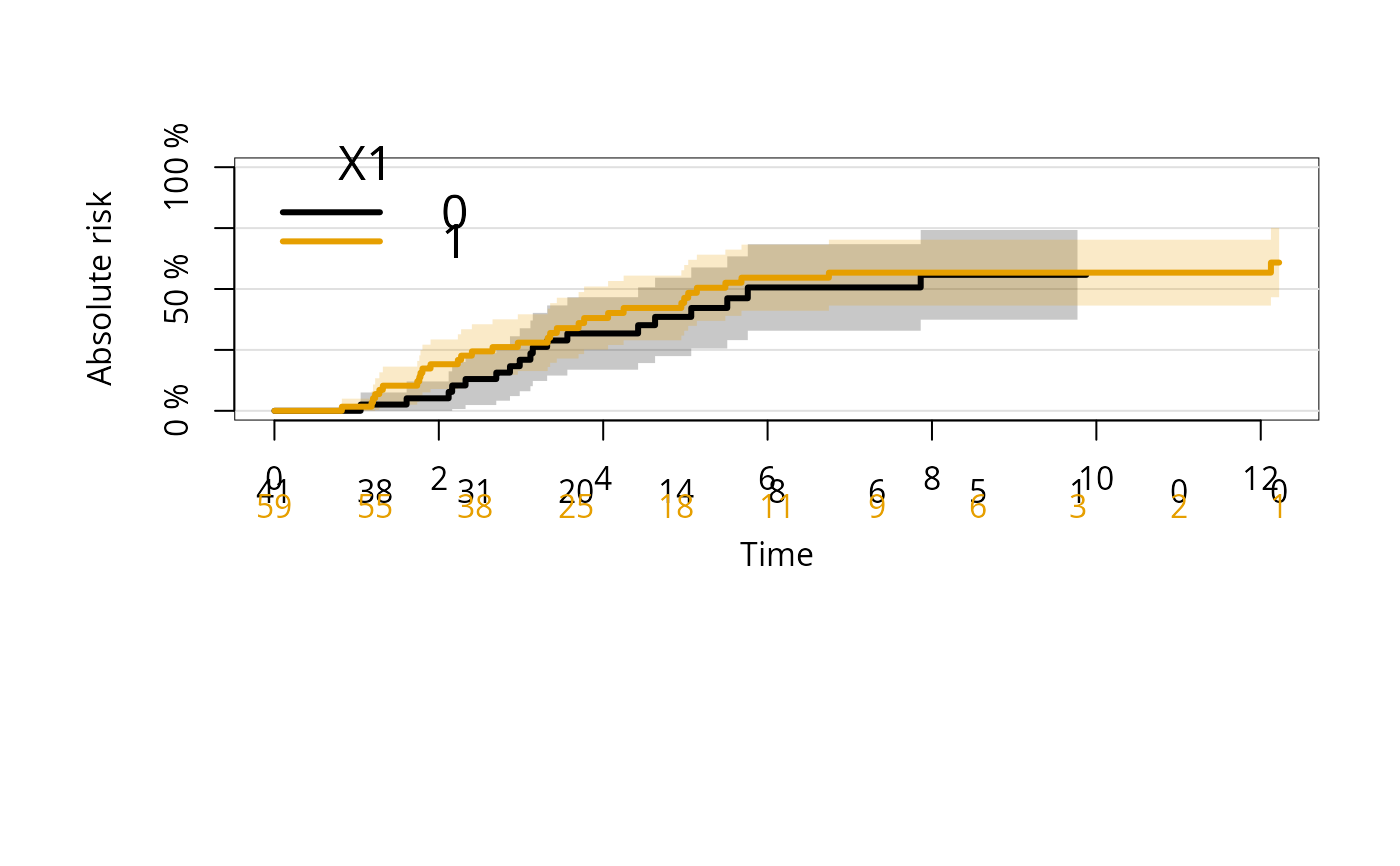
### stratified Aalen-Johansen estimator
ajfitX1 <- prodlim(Hist(time, event) ~ X1, data = datCR)
plot(ajfitX1)
 ## add total number at-risk to a stratified curve
ttt = 1:10
plot(ajfitX1,atrisk.at=ttt,col=2:3)
plot(ajfit,add=TRUE,col=1)
atRisk(ajfit,newdata=datCR,col=1,times=ttt,line=3,labels="Total")
## add total number at-risk to a stratified curve
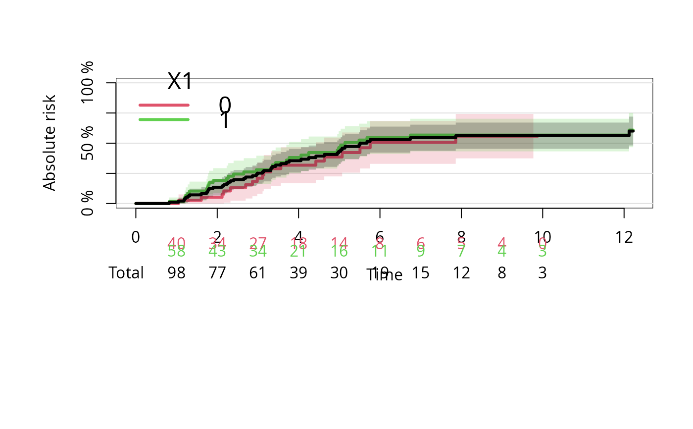
ttt = 1:10
plot(ajfitX1,atrisk.at=ttt,col=2:3)
plot(ajfit,add=TRUE,col=1)
atRisk(ajfit,newdata=datCR,col=1,times=ttt,line=3,labels="Total")
 #> [[1]]
#> NULL
#>
## stratified Aalen-Johansen estimator in nearest neighborhoods
## of a continuous variable
ajfitX <- prodlim(Hist(time, event) ~ X1+X2, data = datCR)
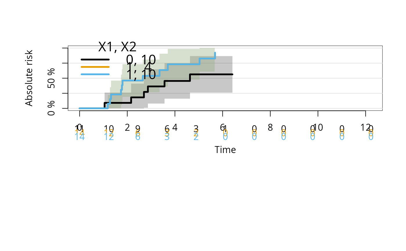
plot(ajfitX,newdata=data.frame(X1=c(1,1,0),X2=c(4,10,10)))
#> [[1]]
#> NULL
#>
## stratified Aalen-Johansen estimator in nearest neighborhoods
## of a continuous variable
ajfitX <- prodlim(Hist(time, event) ~ X1+X2, data = datCR)
plot(ajfitX,newdata=data.frame(X1=c(1,1,0),X2=c(4,10,10)))
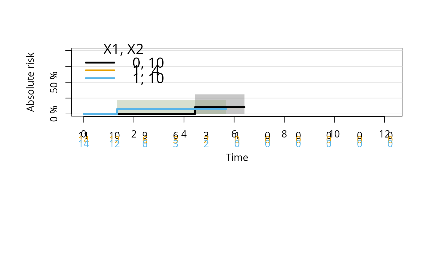
 plot(ajfitX,newdata=data.frame(X1=c(1,1,0),X2=c(4,10,10)),cause=2)
 ## stacked plot
plot(ajfitX,
newdata=data.frame(X1=0,X2=0.1),
cause="stacked",
legend.title="X1=0,X2=0.1",
legend.legend=paste("cause:",getStates(ajfitX$model.response)),
plot.main="Subject specific stacked plot")
## stacked plot
plot(ajfitX,
newdata=data.frame(X1=0,X2=0.1),
cause="stacked",
legend.title="X1=0,X2=0.1",
legend.legend=paste("cause:",getStates(ajfitX$model.response)),
plot.main="Subject specific stacked plot")