Restricted permutations; using the permute package

Gavin L. Simpson

2026-02-18

Introduction

In classical frequentist statistics, the significance of a relationship or model is determined by reference to a null distribution for the test statistic. This distribution is derived mathematically and the probability of achieving a test statistic as large or larger than the observed statistic if the null hypothesis were true is looked-up from this null distribution. In deriving this probability, some assumptions about the data or the errors are made. If these assumptions are violated, then the validity of the derived $p$-value may be questioned.

An alternative to deriving the null distribution from theory is to generate a null distribution of the test statistic by randomly shuffling the data in some manner, refitting the model and deriving values for the test statistic for the permuted data. The level of significance of the test can be computed as the proportion of values of the test statistic from the null distribution that are equal to or larger than the observed value.

In many data sets, simply shuffling the data at random is inappropriate; under the null hypothesis, the data may not ne freely exchangeable, for example if there is temporal or spatial correlation, or the samples are clustered in some way, such as multiple samples collected from each of a number of fields. The permute package was designed to provide facilities for generating these restricted permutations for use in randomisation tests. permute takes as its motivation the permutation schemes originally available in Canoco version 3.1 (Braak 1990), which employed the cyclic- or toroidal-shifts suggested by Besag and Clifford (1989).

Simple randomisation

As an illustration of both randomisation and simple usage of the permute package we consider a small data set of mandible length measurements on specimens of the golden jackal (Canis aureus) from the British Museum of Natural History, London, UK. These data were collected as part of a study comparing prehistoric and modern canids (Higham, Kijngam, and Manly 1980), and were analysed by Manly (2007). There are ten measurements of mandible length on both male and female specimens. The data are available in the jackal data frame supplied with permute.

library("permute")
data(jackal)
jackal

##    Length    Sex
## 1     120   Male
## 2     107   Male
## 3     110   Male
## 4     116   Male
## 5     114   Male
## 6     111   Male
## 7     113   Male
## 8     117   Male
## 9     114   Male
## 10    112   Male
## 11    110 Female
## 12    111 Female
## 13    107 Female
## 14    108 Female
## 15    110 Female
## 16    105 Female
## 17    107 Female
## 18    106 Female
## 19    111 Female
## 20    111 Female

The interest is whether there is a difference in the mean mandible length between male and female golden jackals. The null hypothesis is that there is zero difference in mandible length between the two sexes or that females have larger mandibles. The alternative hypothesis is that males have larger mandibles. The usual statistical test of this hypothesis is a one-sided $t$ test, which can be applied using t.test()

jack.t <- t.test(Length ~ Sex, data = jackal, var.equal = TRUE,
                 alternative = "greater")
jack.t

## 
##  Two Sample t-test
## 
## data:  Length by Sex
## t = 3.4843, df = 18, p-value = 0.001324
## alternative hypothesis: true difference in means between group Male and group Female is greater than 0
## 95 percent confidence interval:
##  2.411156      Inf
## sample estimates:
##   mean in group Male mean in group Female 
##                113.4                108.6

The observed $t$ is 3.484 with 18 df. The probability of observing a value this large or larger if the null hypothesis were true is 0.0013. Several assumptions have been made in deriving this $p$-value, namely

• random sampling of individuals from the populations of interest,
• equal population standard deviations for males and females, and
• that the mandible lengths are normally distributed within the sexes.

Assumption 1 is unlikely to be valid for museum specimens such as these, that have been collected in some unknown manner. Assumption 2 may be valid, Fisher’s $F$-test and a Fligner-Killeen test both suggest that the standard deviations of the two populations do not differ significantly

var.test(Length ~ Sex, data = jackal)
fligner.test(Length ~ Sex, data = jackal)

This assumption may be relaxed using var.equal = FALSE (the default) in the call to t.test(), to employ Welch’s modification for unequal variances. Assumption 3 may be valid, but with such a small sample we are unable to reliably test this.

A randomisation test of the same hypothesis can be performed by randomly allocating ten of the mandible lengths to the male group and the remaining lengths to the female group. This randomisation is justified under the null hypothesis because the observed difference in mean mandible length between the two sexes is just a typical value for the difference in a sample if there were no difference in the population. An appropriate test statistic needs to be selected. We could use the $t$ statistic as derived in the $t$-test. Alternatively, we could base our randomisation test on the difference of means $D_i$ (male - female).

The main function in permute for providing random permutations is shuffle(). We can write our own randomisation test for the jackal data by first creating a function to compute the difference of means for two groups

meanDif <- function(x, grp) {
 mean(x[grp == "Male"]) - mean(x[grp == "Female"])
}

which can be used in a simple for() loop to generate the null distribution for the difference of means. First, we allocate some storage to hold the null difference of means; here we use 4999 random permutations so allocate a vector of length 5000. Then we iterate, randomly generating an ordering of the Sex vector and computing the difference of means for that permutation.

Djackal <- numeric(length = 5000)
N <- nrow(jackal)
set.seed(42)
for(i in seq_len(length(Djackal) - 1)) {
    perm <- shuffle(N)
    Djackal[i] <- with(jackal, meanDif(Length, Sex[perm]))
}
Djackal[5000] <- with(jackal, meanDif(Length, Sex))

The observed difference of means was added to the null distribution, because under the null hypothesis the observed allocation of mandible lengths to male and female jackals is just one of the possible random allocations.

The null distribution of $D_i$ can be visualised using a histogram, as shown in Figure~@ref{draw_hist_jackal}. The observed difference of means (4.8) is indicated by the red tick mark.

hist(Djackal, main = "",
     xlab = expression("Mean difference (Male - Female) in mm"))
rug(Djackal[5000], col = "red", lwd = 2)

The number of values in the randomisation distribution equal to or larger than the observed difference is

(Dbig <- sum(Djackal >= Djackal[5000]))

## [1] 12

giving a permutational $p$-value of

Dbig / length(Djackal)

## [1] 0.0024

which is comparable with that determined from the frequentist $t$-test, and indicates strong evidence against the null hypothesis of no difference.

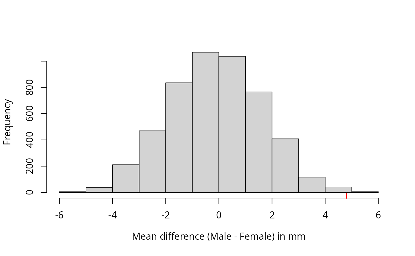
Distribution of the difference of mean mandible length in random allocations, ten to each sex.

In total there $^{20}C_{10} = 184,756$ possible allocations of the 20 observations to two groups of ten

choose(20, 10)

## [1] 184756

so we have only evaluated a small proportion of these in the randomisation test.

The main workhorse function we used above was shuffle(). In this example, we could have used the base R function sample() to generate the randomised indices perm that were used to permute the Sex factor. Where shuffle() comes into it’s own is for generating permutation indices from restricted permutation designs.

The shuffle() and shuffleSet() functions

In the previous section I introduced the shuffle() function to generate permutation indices for use in a randomisation test. Now we will take a closer look at shuffle() and explore the various restricted permutation designs from which it can generate permutation indices.

shuffle() has two arguments:

1. n, the number of observations in the data set to be permuted, and
2. control, a list that defines the permutation design describing how the samples should be permuted.

args(shuffle)

## function (n, control = how()) 
## NULL

A series of convenience functions are provided that allow the user to set-up even quite complex permutation designs with little effort. The user only needs to specify the aspects of the design they require and the convenience functions ensure all configuration choices are set and passed on to shuffle(). The main convenience function is how(), which returns a list specifying all the options available for controlling the sorts of permutations returned by shuffle().

str(how())

## List of 12
##  $ within     :List of 6
##   ..$ type    : chr "free"
##   ..$ constant: logi FALSE
##   ..$ mirror  : logi FALSE
##   ..$ ncol    : NULL
##   ..$ nrow    : NULL
##   ..$ call    : language Within()
##   ..- attr(*, "class")= chr "Within"
##  $ plots      :List of 7
##   ..$ strata    : NULL
##   ..$ type      : chr "none"
##   ..$ mirror    : logi FALSE
##   ..$ ncol      : NULL
##   ..$ nrow      : NULL
##   ..$ plots.name: chr "NULL"
##   ..$ call      : language Plots()
##   ..- attr(*, "class")= chr "Plots"
##  $ blocks     : NULL
##  $ nperm      : num 199
##  $ complete   : logi FALSE
##  $ maxperm    : num 9999
##  $ minperm    : num 5040
##  $ all.perms  : NULL
##  $ make       : logi TRUE
##  $ observed   : logi FALSE
##  $ blocks.name: chr "NULL"
##  $ call       : language how()
##  - attr(*, "class")= chr "how"

The defaults describe a random permutation design where all objects are freely exchangeable. Using these defaults, shuffle(10) amounts to sample(1:10, 10, replace = FALSE):

set.seed(2)
(r1 <- shuffle(10))

##  [1]  5  6  9  1 10  7  4  8  3  2

set.seed(2)
(r2 <- sample(1:10, 10, replace = FALSE))

##  [1]  5  6  9  1 10  7  4  8  3  2

all.equal(r1, r2)

## [1] TRUE

Generating restricted permutations

Several types of permutation are available in permute:

• Free permutation of objects
• Time series or line transect designs, where the temporal or spatial ordering is preserved.
• Spatial grid designs, where the spatial ordering is preserved in both coordinate directions
• Permutation of plots or groups of samples.
• Blocking factors which restrict permutations to within blocks. The preceding designs can be nested within blocks.

The first three of these can be nested within the levels of a factor or to the levels of that factor, or to both. Such flexibility allows the analysis of split-plot designs using permutation tests, especially when combined with blocks.

how() is used to set up the design from which shuffle() will draw a permutation. how() has two main arguments that specify how samples are permuted within plots of samples or at the plot level itself. These are within and plots. Two convenience functions, Within() and Plots() can be used to set the various options for permutation. Blocks operate at the uppermost level of this hierarchy; blocks define groups of plots, each of which may contain groups of samples.

For example, to permute the observations 1:10 assuming a time series design for the entire set of observations, the following control object would be used

set.seed(4)
x <- 1:10
CTRL <- how(within = Within(type = "series"))
perm <- shuffle(10, control = CTRL)
perm

##  [1]  9 10  1  2  3  4  5  6  7  8

x[perm] ## equivalent

##  [1]  9 10  1  2  3  4  5  6  7  8

It is assumed that the observations are in temporal or transect order. We only specified the type of permutation within plots, the remaining options were set to their defaults via Within().

A more complex design, with three plots, and a 3 by 3 spatial grid arrangement within each plot can be created as follows

set.seed(4)
plt <- gl(3, 9)
CTRL <- how(within = Within(type = "grid", ncol = 3, nrow = 3),
            plots = Plots(strata = plt))
perm <- shuffle(length(plt), control = CTRL)
perm

##  [1]  1  2  3  4  5  6  7  8  9 10 11 12 13 14 15 16 17 18 25 26 27 19 20 21 22
## [26] 23 24

Visualising the permutation as the 3 matrices may help illustrate how the data have been shuffled

## Original
lapply(split(seq_along(plt), plt), matrix, ncol = 3)

## $`1`
##      [,1] [,2] [,3]
## [1,]    1    4    7
## [2,]    2    5    8
## [3,]    3    6    9
## 
## $`2`
##      [,1] [,2] [,3]
## [1,]   10   13   16
## [2,]   11   14   17
## [3,]   12   15   18
## 
## $`3`
##      [,1] [,2] [,3]
## [1,]   19   22   25
## [2,]   20   23   26
## [3,]   21   24   27

## Shuffled
lapply(split(perm, plt), matrix, ncol = 3)

## $`1`
##      [,1] [,2] [,3]
## [1,]    1    4    7
## [2,]    2    5    8
## [3,]    3    6    9
## 
## $`2`
##      [,1] [,2] [,3]
## [1,]   10   13   16
## [2,]   11   14   17
## [3,]   12   15   18
## 
## $`3`
##      [,1] [,2] [,3]
## [1,]   25   19   22
## [2,]   26   20   23
## [3,]   27   21   24

In the first grid, the lower-left corner of the grid was set to row 2 and column 2 of the original, to row 1 and column 2 in the second grid, and to row 3 column 2 in the third grid.

To have the same permutation within each level of plt, use the constant argument of the Within() function, setting it to TRUE

set.seed(4)
CTRL <- how(within = Within(type = "grid", ncol = 3, nrow = 3,
                            constant = TRUE),
            plots = Plots(strata = plt))
perm2 <- shuffle(length(plt), control = CTRL)
lapply(split(perm2, plt), matrix, ncol = 3)

## $`1`
##      [,1] [,2] [,3]
## [1,]    1    4    7
## [2,]    2    5    8
## [3,]    3    6    9
## 
## $`2`
##      [,1] [,2] [,3]
## [1,]   10   13   16
## [2,]   11   14   17
## [3,]   12   15   18
## 
## $`3`
##      [,1] [,2] [,3]
## [1,]   19   22   25
## [2,]   20   23   26
## [3,]   21   24   27

Generating sets of permutations with shuffleSet()

There are several reasons why one might wish to generate a set of $n$ permutations instead of repeatedly generating permutations one at a time. Interpreting the permutation design happens each time shuffle() is called. This is an unnecessary computational burden, especially if you want to perform tests with large numbers of permutations. Furthermore, having the set of permutations available allows for expedited use with other functions, they can be iterated over using for loops or the apply family of functions, and the set of permutations can be exported for use outside of R.

The shuffleSet() function allows the generation of sets of permutations from any of the designs available in permute. shuffleSet() takes an additional argument to that of shuffle(), nset, which is the number of permutations required for the set. nset can be missing, in which case the number of permutations in the set is looked for in the object passed to control; using this, the desired number of permutations can be set at the time the design is created via the nperm argument of how(). For example,

how(nperm = 10, within = Within(type = "series"))

Internally, shuffle() and shuffleSet() are very similar, with the major difference being that shuffleSet() arranges repeated calls to the workhorse permutation-generating functions, only incurring the overhead associated with interpreting the permutation design once. shuffleSet() returns a matrix where the rows represent different permutations in the set.

As an illustration, consider again the simple time series example from earlier. Here I generate a set of 5 permutations from the design, with the results returned as a matrix

set.seed(4)
CTRL <- how(within = Within(type = "series"))
pset <- shuffleSet(10, nset = 5, control = CTRL)
pset

## No. of Permutations: 5
## No. of Samples: 10 (Sequence)
## 
##     1  2  3 4 5  6  7 8 9 10
## p1  9 10  1 2 3  4  5 6 7  8
## p2  4  5  6 7 8  9 10 1 2  3
## p3 10  1  2 3 4  5  6 7 8  9
## p4  8  9 10 1 2  3  4 5 6  7
## p5  5  6  7 8 9 10  1 2 3  4

It is worth taking a moment to explain what has happened here, behind the scenes. There are only 10 unique orderings (including the observed) in the set of permutations for this design. Such a small set of permutations triggers¹ the generation of the entire set of permutations. From this set, shuffleSet() samples at random nset permutations. Hence the same number of random values has been generated via the pseudo-random number generator in R but we ensure a set of unique permutations is drawn, rather than randomly sample from a small set.

Defining permutation designs

In this section I give examples how various permutation designs can be specified using how(). It is not the intention to provide exhaustive coverage of all possible designs that can be produced; such a list would be tedious to both write and read. Instead, the main features and options will be described through a series of examples. The reader should then be able to put together the various options to create the exact structure required.

Set the number of permutations

It may be useful to specify the number of permutations required in a permutation test alongside the permutation design. This is done via the nperm argument, as seen earlier. If nothing else is specified

how(nperm = 999)

would indicate 999 random permutations where the samples are all freely exchangeable.

One advantage of using nperm is that shuffleSet() will use this if the nset argument is not specified. Additionally, shuffleSet() will check to see if the desired number of permutations is possible given the data and the requested design. This is done via the function check(), which is discussed later.

The levels of the permutation hierarchy

There are three levels at which permutations can be controlled in permute. The highest level of the hierarchy is the block level. Blocks are defined by a factor variable. Blocks restrict permutation of samples to within the levels of this factor; samples are never swapped between blocks.

The plot level sits below blocks. Plots are defined by a factor and group samples in the same way as blocks. As such, some permutation designs can be initiated using a factor at the plot level or the same factor at the block level. The major difference between blocks and plots is that plots can also be permuted, whereas blocks are never permuted.

The lowest level of a permutation design in the permute hierarchy is known as within, and refers to samples nested within plots. If there are no plots or blocks, how samples are permuted at the within level applies to the entire data set.

Permuting samples at the lowest level

How samples at the within level are permuted is configured using the Within() function. It takes the following arguments

## function (type = c("free", "series", "grid", "none"), constant = FALSE, 
##     mirror = FALSE, ncol = NULL, nrow = NULL) 
## NULL

type

controls how the samples at the lowest level are permuted. The default is to form unrestricted permutations via option "type". Options "series" and "grid" form restricted permutations via cyclic or toroidal shifts, respectively. The former is useful for samples that are a time series or line-transect, whilst the latter is used for samples on a regular spatial grid. The final option, "none", will result in the samples at the lowest level not being permuted at all. This option is only of practical use when there are plots within the permutation/experimental design[^As blocks are never permuted, using type = "none" at the within level is also of no practical use.].

constant

this argument only has an effect when there are plots in the design[^Owing to the current implementation, whilst this option could also be useful when blocks to define groups of samples, it will not have any influence over how permutations are generated. As such, only use blocks for simple blocking structures and use plots if you require greater control of the permutations at the group (i.e. plot) level.]. constant = TRUE stipulates that each plot should have the same within-plot permutation. This is useful for example when you have time series of observations from several plots. If all plots were sampled at the same time points, it can be argued that at the plot level, the samples experienced the same time and hence the same permutation should be used within each plot.

mirror

when type is "series" or "grid", argument "mirror" controls whether permutations are taken from the mirror image of the observed ordering in space or time. Consider the sequence 1, 2, 3, 4. The relationship between observations is also preserved if we reverse the original ordering to 4, 3, 2, 1 and generate permutations from both these orderings. This is what happens when mirror = TRUE. For time series, the reversed ordering 4, 3, 2, 1 would imply an influence of observation 4 on observation 3, which is implausible. For spatial grids or line transects, however, this is a sensible option, and can significantly increase the number of possible permutations[^Setting mirror = TRUE will double or quadruple the set of permutations for "series" or "grid" permutations, respectively, as long as there are more than two time points or columns in the grid.].

ncol, nrow

define the dimensions of the spatial grid.

How Within() is used has already been encountered in earlier sections of this vignette; the function is used to supply a value to the within argument of how(). You may have noticed that all the arguments of Within() have default values? This means that the user need only supply a modified value for the arguments they wish to change. Also, arguments that are not relevant for the type of permutation stated are simply ignored; nrow and ncol, for example, could be set to any value without affecting the permutation design if type != "grid"[^No warnings are currently given if incompatible arguments are specified; they are ignored, but may show up in the printed output. This infelicity will be removed prior to permute version 1.0-0 being released.].

Permuting samples at the Plot level

Permutation of samples at the plot level is configured via the Plots() function. As with Within(), Plots() is supplied to the plots argument of how(). Plots() takes many of the same arguments as Within(), the two differences being strata, a factor variable that describes the grouping of samples at the plot level, and the absence of a constant argument. As the majority of arguments are similar between Within() and Plots(), I will not repeat the details again, and only describe the strata argument

strata

a factor variable. strata describes the grouping of samples at the plot level, where samples from the same plot are take the same level of the factor.

When a plot-level design is specified, samples are never permuted between plots, only within plots if they are permuted at all. Hence, the type of permutation within the plots is controlled by Within(). Note also that with Plots(), the way the individual plots are permuted can be from any one of the four basic permutation types; "none", "free", "series", and "grid", as described above. To permute the plots only (i.e. retain the ordering of the samples within plots), you also need to specify Within(type = "none", ...) as the default in Within() is type = "free". The ability to permute the plots whilst preserving the within-plot ordering is an impotant feature in testing explanatory factors at the whole-plot level in split-plot designs and in multifactorial analysis of variance (Braak and Šmilauer 2012).

Specifying blocks; the top of the permute hierarchy

In constrast to the within and plots levels, the blocks level is simple to specify; all that is required is an indicator variable the same length as the data. Usually this is a factor, but how() will take anything that can be coerced to a factor via as.factor().

It is worth repeating what the role of the block-level structure is; blocks simply restrict permutation to within, and never between, blocks, and blocks are never permuted. This is reflected in the implementation; the split-apply-combine paradigm is used to split on the blocking factor, the plot- and within-level permutation design is applied separately to each block, and finally the sets of permutations for each block are recombined.

Examples

To do.

Using permute in R functions

permute originally started life as a set of functions contained within the vegan package (Oksanen et al. 2013) designed to provide a replacement for the permuted.index() function. From these humble origins, I realised other users and package authors might want to make use of the code I was writing and so Jari oksanen, the maintainer of vegan, and I decided to spin off the code into the permute package. Hence from the very beginning, permute was intended for use both by users, to defining permutation designs, and by package authors, with which to implement permutation tests within their packages.

In the previous sections, I described the various user-facing functions that are employed to set up permutation designs and generate permutations from these. Here I will outline how package authors can use functionality in the permute package to implement permutation tests.

In Section~@ref{sec:simple} I showed how a permutation test function could be written using the shuffle() function and allowing the user to pass into the test function an object created with how(). As mentioned earlier, it is more efficient to generate a set of permutations via a call to shuffleSet() than to repeatedly call shuffle() and large number of times. Another advantage of using shuffleSet() is that once the set of permutations has been created, parallel processing can be used to break the set of permutations down into smaller chunks, each of which can be worked on simultaneously. As a result, package authors are encouraged to use shuffleSet() instead of the simpler shuffle().

To illustrate how to use permute in R functions, I’ll rework the permutation test I used for the jackal data earlier in Section~@ref{sec:simple}.

pt.test <- function(x, group, nperm = 199) {
    ## mean difference function
    meanDif <- function(i, x, grp) {
        grp <- grp[i]
        mean(x[grp == "Male"]) - mean(x[grp == "Female"])
    }
    ## check x and group are of same length
    stopifnot(all.equal(length(x), length(group)))
    ## number of observations
    N <- nobs(x)
    ## generate the required set of permutations
    pset <- shuffleSet(N, nset = nperm)
    ## iterate over the set of permutations applying meanDif
    D <- apply(pset, 1, meanDif, x = x, grp = group)
    ## add on the observed mean difference
    D <- c(meanDif(seq_len(N), x, group), D)
    ## compute & return the p-value
    Ds <- sum(D >= D[1]) # how many >= to the observed diff?
    Ds / (nperm + 1)     # what proportion of perms is this (the pval)?
}

The commented function should be reasonably self explanatory. I’ve altered the in-line version of the meanDif() function to take a vector of permutation indices i as the first argument, and internally the grp vector is permuted according to i. The other major change is that shuffleSet() is used to generate a set of permutations, which are then iterated over using apply().

In use we see

set.seed(42) ## same seed as earlier
pval <- with(jackal, pt.test(Length, Sex, nperm = 4999))
pval

## [1] 0.0024

which nicely agrees with the test we did earlier by hand.

Iterating over a set of permutation indices also means that adding parallel processing of the permutations requires only trivial changes to the main function code. As an illustration, below I show a parallel version of pt.test()

ppt.test <- function(x, group, nperm = 199, cores = 2) {
    ## mean difference function
    meanDif <- function(i, .x, .grp) {
        .grp <- .grp[i]
        mean(.x[.grp == "Male"]) - mean(.x[.grp == "Female"])
    }
    ## check x and group are of same length
    stopifnot(all.equal(length(x), length(group)))
    ## number of observations
    N <- nobs(x)
    ## generate the required set of permutations
    pset <- shuffleSet(N, nset = nperm)
    if (cores > 1) {
        ## initiate a cluster
        cl <- makeCluster(cores)
        on.exit(stopCluster(cl = cl))
        ## iterate over the set of permutations applying meanDif
        D <- parRapply(cl, pset, meanDif, .x = x, .grp = group)
    } else {
        D <- apply(pset, 1, meanDif, .x = x, .grp = group)
    }
    ## add on the observed mean difference
    D <- c(meanDif(seq_len(N), x, group), D)
    ## compute & return the p-value
    Ds <- sum(D >= D[1]) # how many >= to the observed diff?
    Ds / (nperm + 1)     # what proportion of perms is this (the pval)?
}

In use we observe

require("parallel")
set.seed(42)
system.time(ppval <- ppt.test(jackal$Length, jackal$Sex, nperm = 9999,
                              cores = 2))

##    user  system elapsed 
##   0.069   0.004   0.512

ppval

## [1] 0.0018

In this case there is little to be gained by splitting the computations over two CPU cores

set.seed(42)
system.time(ppval2 <- ppt.test(jackal$Length, jackal$Sex, nperm = 9999,
                               cores = 1))

##    user  system elapsed 
##   0.234   0.001   0.235

ppval2

## [1] 0.0018

The cost of setting up and managing the parallel processes, and recombining the separate sets of results almost negates the gain in running the permutations in parallel. Here, the computations involved in meanDif() are trivial and we would expect greater efficiencies from running the permutations in parallel for more complex analyses.

Accesing and changing permutation designs

The object created by how() is a relatively simple list containing the settings for the specified permutation design. As such one could use the standard subsetting and replacement functions in base R to alter components of the list. This is not recommended, however, as the internal structure of the list returned by how() may change in a later version of permute. Furthermore, to facilitate the use of update() at the user-level to alter the permutation design in a user-friendly way, the matched how() call is stored within the list along with the matched calls for any Within() or Plots() components. These matched calls need to be updated too if the list describing the permutation design is altered. To allow function writers to access and alter permutation designs, permute provides a series of extractor and replacement functions that have the forms getFoo() and setFoo<-(), respectively,where Foo is replaced by a particular component to be extracted or replaced.

The getFoo() functions provided by permute are

getWithin(), getPlots(), getBlocks()

these extract the details of the within-, plots-, and blocks-level components of the design. Given the current design (as of permute version 0.8-0), the first two of these return lists with classes "Within" and "Plots", respectively, whilst getBlocks() returns the block-level factor.

getStrata()

returns the factor describing the grouping of samples at the plots or blocks levels, as determined by the value of argument which.

getType()

returns the type of permutation of samples at the within or plots levels, as determined by the value of argument which.

getMirror()

returns a logical, indicating whether permutations are drawn from the mirror image of the observed ordering at the within or plots levels, as determined by the value of argument which.

getConstant()

returns a logical, indicating whether the same permutation of samples, or a different permutation, is used within each of the plots.

getRow(), getCol(), getDim()

return dimensions of the spatial grid of samples at the plots or blocks levels, as determined by the value of argument which.

getNperm(), getMaxperm(), getMinperm()

return numerics for the stored number of permutations requested plus two triggers used when checking permutation designs via check().

getComplete()

returns a logical, indicating whether complete enumeration of the set of permutations was requested.

getMake()

returns a logical, indicating whether the entire set of permutations should be produced or not.

getObserved()

returns a logical, which indicates whether the observed permutation (ordering of samples) is included in the entire set of permutation generated by allPerms().

getAllperms()

extracts the complete set of permutations if present. Returns NULL if the set has not been generated.

The available setFoo()<- functions are

setPlots<-(), setWithin<-()

replaces the details of the within-, and plots-, components of the design. The replacement object must be of class "Plots" or "Within", respectively, and hence is most usefully used in combination with the Plots() or Within() constructor functions.

setBlocks<-()

replaces the factor that partitions the observations into blocks. value can be any R object that can be coerced to a factor vector via as.factor().

setStrata<-()

replaces either the blocks or strata components of the design, depending on what class of object setStrata<-() is applied to. When used on an object of class "how", setStrata<-() replaces the blocks component of that object. When used on an object of class "Plots", setStrata<-() replaces the strata component of that object. In both cases a factor variable is required and the replacement object will be coerced to a factor via as.factor() if possible.

setType<-()

replaces the type component of an object of class "Plots" or "Within" with a character vector of length one. Must be one of the available types: "none", "free", "series", or "grid".

setMirror<-()

replaces the mirror component of an object of class "Plots" or "Within" with a logical vector of length one.

setConstant<-()

replaces the constant component of an object of class "Within" with a logical vector of length one.

setRow<-(), setCol<-(), setDim<-()

replace one or both of the spatial grid dimensions of an object of class "Plots" or "Within" with am integer vector of length one, or, in the case of setDim<-(), of length 2.

setNperm<-(), setMinperm<-(), setMaxperm<-()

update the stored values for the requested number of permutations and the minimum and maximum permutation thresholds that control whether the entire set of permutations is generated instead of nperm permutations.

setAllperms<-()

assigns a matrix of permutation indices to the all.perms component of the design list object.

setComplete<-()

updates the status of the complete setting. Takes a logical vector of length 1 or any object coercible to such.

setMake<-()

sets the indicator controlling whether the entrie set of permutations is generated during checking of the design via check(). Takes a logical vector of length 1 or any object coercible to such.

setObserved<-()

updates the indicator of whether the observed ordering is included in the set of all permutations should they be generated. Takes a logical vector of length 1 or any object coercible to such.

Examples

I illustrate the behaviour of the getFoo() and setFoo<-() functions through a couple of simple examples. Firstly, generate a design object

hh <- how()

This design is one of complete randomization, so all of the settings in the object take their default values. The default number of permutations is currently 199, and can be extracted using getNperm()

getNperm(hh)

## [1] 199

The corresponding replacement function can be use to alter the number of permutations after the design has been generated. To illustrate a finer point of the behaviour of these replacement functions, compare the matched call stored in hh before and after the number of permutations is changed

getCall(hh)

## how()

setNperm(hh) <- 999
getNperm(hh)

## [1] 999

getCall(hh)

## how(nperm = 999)

Note how the call component has been altered to include the argument pair nperm = 999, hence if this call were evaluated, the resulting object would be a copy of hh.

As a more complex example, consider the following design consisting of 5 blocks, each containing 2 plots of 5 samples each. Hence there are a total of 10 plots. Both the plots and within-plot sample are time series. This design can be created using

hh <- how(within = Within(type = "series"),
          plots = Plots(type = "series", strata = gl(10, 5)),
          blocks = gl(5, 10))

To alter the design at the plot or within-plot levels, it is convenient to extract the relevant component using getPlots() or getWithin(), update the extracted object, and finally use the updated object to update hh. This process is illustrated below in order to change the plot-level permutation type to "free"

pl <- getPlots(hh)
setType(pl) <- "free"
setPlots(hh) <- pl

We can confirm this has been changed by extracting the permutation type for the plot level

getType(hh, which = "plots")

## [1] "free"

Notice too how the call has been expanded from gl(10, 5) to an integer vector. This expansion is to avoid the obvious problem of locating the objects referred to in the call should the call be re-evaluated later.

getCall(getPlots(hh))

## Plots(strata = c(1L, 1L, 1L, 1L, 1L, 2L, 2L, 2L, 2L, 2L, 3L, 
## 3L, 3L, 3L, 3L, 4L, 4L, 4L, 4L, 4L, 5L, 5L, 5L, 5L, 5L, 6L, 6L, 
## 6L, 6L, 6L, 7L, 7L, 7L, 7L, 7L, 8L, 8L, 8L, 8L, 8L, 9L, 9L, 9L, 
## 9L, 9L, 10L, 10L, 10L, 10L, 10L), type = "free")

At the top level, a user can update the design using update(). Hence the equivalent of the above update is (this time resetting the original type; type = "series")

hh <- update(hh, plots = update(getPlots(hh), type = "series"))
getType(hh, which = "plots")

## [1] "series"

However, this approach is not assured of working within a function because we do not guarantee that components of the call used to create hh can be found from the execution frame where update() is called. To be safe, always use the setFoo<-() replacement functions to update design objects from within your functions.

Computational details

This vignette was built within the following environment:

## ─ Session info ───────────────────────────────────────────────────────────────
##  setting  value
##  version  R version 4.5.1 (2025-06-13)
##  os       Ubuntu 24.04.3 LTS
##  system   x86_64, linux-gnu
##  ui       X11
##  language en
##  collate  C.UTF-8
##  ctype    C.UTF-8
##  tz       Etc/UTC
##  date     2026-02-18
##  pandoc   3.6.3 @ /usr/lib/rstudio-server/bin/quarto/bin/tools/x86_64/ (via rmarkdown)
##  quarto   1.7.31 @ /usr/local/bin/quarto
## 
## ─ Packages ───────────────────────────────────────────────────────────────────
##  ! package     * version date (UTC) lib source
##  P bookdown      0.46    2025-12-05 [?] PRISM (R 4.5.0)
##  P bslib         0.10.0  2026-01-26 [?] PRISM (R 4.5.0)
##  P cachem        1.1.0   2024-05-16 [?] PRISM (R 4.5.0)
##  P cli           3.6.5   2025-04-23 [?] PRISM (R 4.5.0)
##  P desc          1.4.3   2023-12-10 [?] PRISM (R 4.5.0)
##  P digest        0.6.39  2025-11-19 [?] PRISM (R 4.5.0)
##  P evaluate      1.0.5   2025-08-27 [?] PRISM (R 4.5.0)
##  P fastmap       1.2.0   2024-05-15 [?] PRISM (R 4.5.0)
##  P fs            1.6.6   2025-04-12 [?] PRISM (R 4.5.0)
##  P htmltools     0.5.9   2025-12-04 [?] PRISM (R 4.5.0)
##  P jquerylib     0.1.4   2021-04-26 [?] PRISM (R 4.5.0)
##  P jsonlite      2.0.0   2025-03-27 [?] PRISM (R 4.5.0)
##  P knitr         1.51    2025-12-20 [?] PRISM (R 4.5.0)
##  P lifecycle     1.0.5   2026-01-08 [?] PRISM (R 4.5.0)
##    permute     * 0.9-10  2026-02-18 [1] local
##  P pkgdown       2.2.0   2025-11-06 [?] PRISM (R 4.5.0)
##  P R6            2.6.1   2025-02-15 [?] PRISM (R 4.5.0)
##  P ragg          1.5.0   2025-09-02 [?] PRISM (R 4.5.0)
##  P rlang         1.1.7   2026-01-09 [?] PRISM (R 4.5.0)
##  P rmarkdown     2.30    2025-09-28 [?] PRISM (R 4.5.0)
##  P sass          0.4.10  2025-04-11 [?] PRISM (R 4.5.0)
##  P sessioninfo   1.2.3   2025-02-05 [?] PRISM (R 4.5.0)
##  P systemfonts   1.3.1   2025-10-01 [?] PRISM (R 4.5.0)
##  P textshaping   1.0.4   2025-10-10 [?] PRISM (R 4.5.0)
##  P xfun          0.56    2026-01-18 [?] PRISM (R 4.5.0)
##  P yaml          2.3.12  2025-12-10 [?] PRISM (R 4.5.0)
## 
##  [1] /tmp/Rtmp10Yrkz/temp_libpath34a3663b838730
##  [2] /data/user-homes/andrew/Projects/prism-pkgdocs-build/installed-pkgs/2026-02-13/permute_0.9-10_lib
##  [3] /opt/R/4.5.1/lib/R/library
## 
##  * ── Packages attached to the search path.
##  P ── Loaded and on-disk path mismatch.
## 
## ──────────────────────────────────────────────────────────────────────────────

Besag, J., and P. Clifford. 1989. “Generalized Monte Carlo Significance Tests.” Biometrika 76 (4): 633–42.

Braak, C. J. F. ter. 1990. Update Notes: CANOCO Version 3.1. Wageningen: Agricultural Mathematics Group.

Braak, C. J. F. ter, and P. Šmilauer. 2012. Canoco Reference Manual and User’s Guide: Software for Ordination (Version 5.0). Microcomputer Power.

Higham, C. F. W, A. Kijngam, and B. F. J. Manly. 1980. “An Analysis of Prehistoric Canid Remains from Thailand.” Journal of Archaeological Science 7: 149–65.

Manly, B. F. J. 2007. Randomization, Bootstrap and Monte Carlo Methods in Biology. 3rd ed. Boca Raton: Chapman & Hall/CRC.

Oksanen, Jari, F. Guillaume Blanchet, Roeland Kindt, Pierre Legendre, Peter R. Minchin, R. B. O’Hara, Gavin L. Simpson, Peter Solymos, M. Henry H. Stevens, and Helene Wagner. 2013. Vegan: Community Ecology Package. http://vegan.r-forge.r-project.org/.