Slice the likelihood of a clm — slice • ordinal

Slice likelihood and plot the slice. This is usefull for illustrating the likelihood surface around the MLE (maximum likelihood estimate) and provides graphics to substantiate (non-)convergence of a model fit. Also, the closeness of a quadratic approximation to the log-likelihood function can be inspected for relevant parameters. A slice is considerably less computationally demanding than a profile.

Usage

slice(object, ...)

# S3 method for class 'clm'
slice(object, parm = seq_along(par), lambda = 3,
     grid = 100, quad.approx = TRUE, ...)

# S3 method for class 'slice.clm'
plot(x, parm = seq_along(x),
    type = c("quadratic", "linear"), plot.mle = TRUE,
    ask = prod(par("mfcol")) < length(parm) && dev.interactive(), ...)

Arguments

object: for the clm method an object of class "clm", i.e., the result of a call to clm.
x: a slice.clm object, i.e., the result of slice(clm.object).
parm: for slice.clm a numeric or character vector indexing parameters, for plot.slice.clm only a numeric vector is accepted. By default all parameters are selected.
lambda: the number of curvature units on each side of the MLE the slice should cover.
grid: the number of values at which to compute the log-likelihood for each parameter.
quad.approx: compute and include the quadratic approximation to the log-likelihood function?
type: "quadratic" plots the log-likelihood function which is approximately quadratic, and "linear" plots the signed square root of the log-likelihood function which is approximately linear.
plot.mle: include a vertical line at the MLE (maximum likelihood estimate) when type = "quadratic"? Ignored for type = "linear".
ask: logical; if TRUE, the user is asked before each plot, see par(ask=.).
...: further arguments to plot.default for the plot method. Not used in the slice method.

Value

The slice method returns a list of data.frames with one data.frame for each parameter slice. Each data.frame contains in the first column the values of the parameter and in the second column the values of the (positive) log-likelihood "logLik". A third column is present if quad.approx = TRUE and contains the corresponding quadratic approximation to the log-likelihood. The original model fit is included as the attribute "original.fit".

The plot method produces a plot of the likelihood slice for each parameter.

Author

Rune Haubo B Christensen

Examples


## fit model:
fm1 <- clm(rating ~ contact + temp, data = wine)
## slice the likelihood:
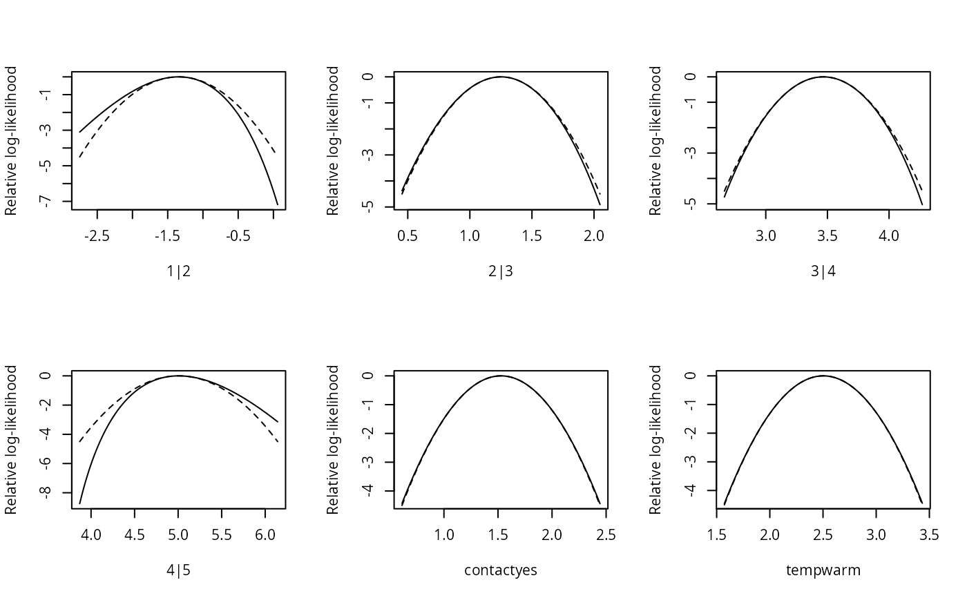
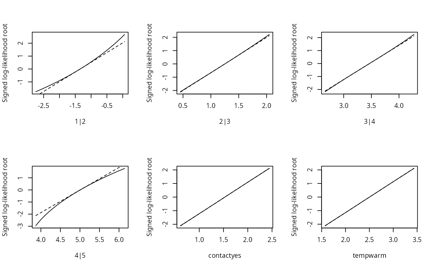
sl1 <- slice(fm1)

## three different ways to plot the slices:
par(mfrow = c(2,3))
plot(sl1)

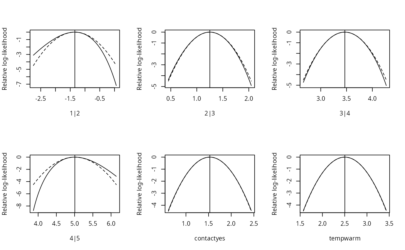plot(sl1, type = "quadratic", plot.mle = FALSE)

plot(sl1, type = "linear")


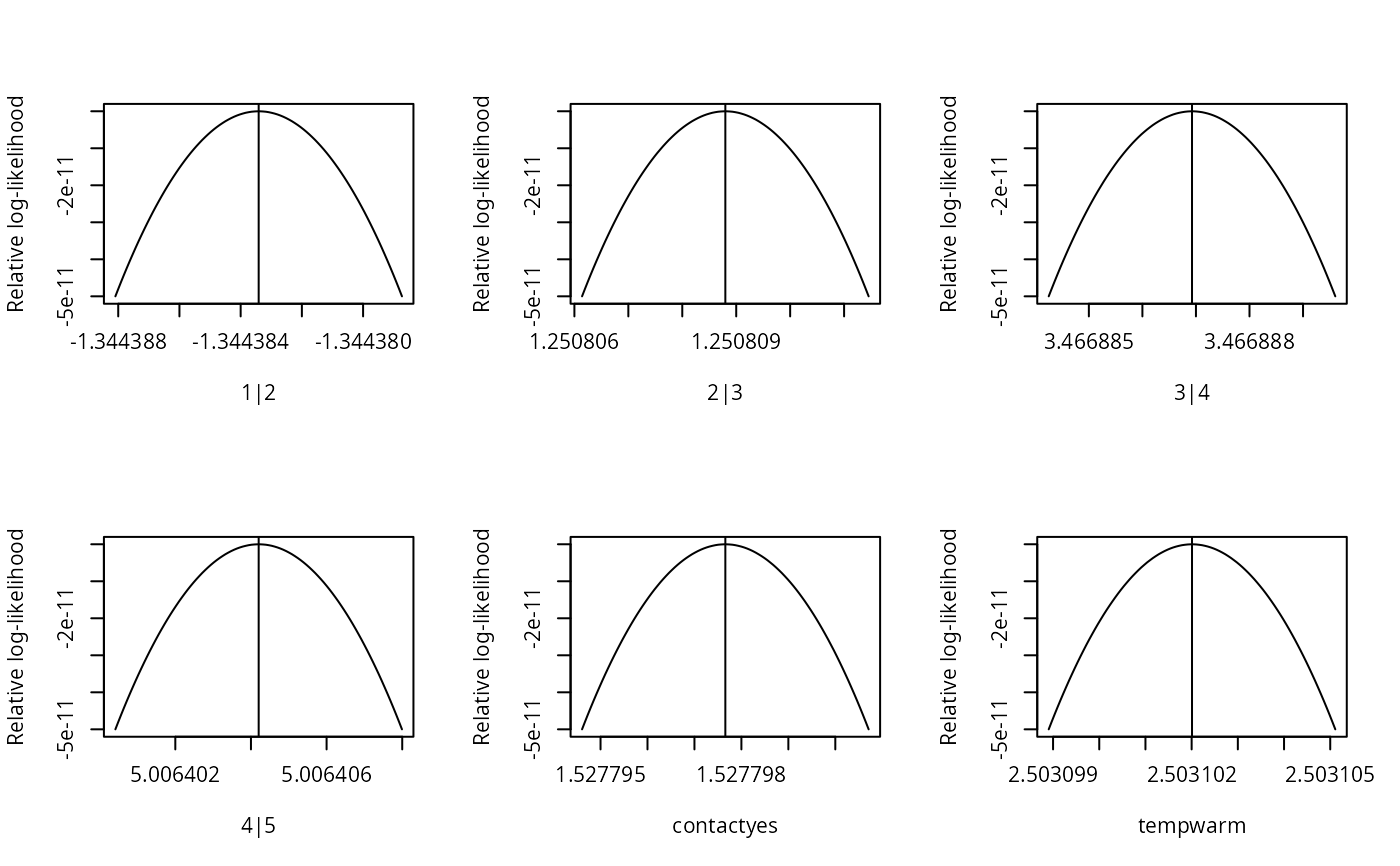
## Verify convergence to the optimum:
sl2 <- slice(fm1, lambda = 1e-5, quad.approx = FALSE)
plot(sl2)