Cumulative Link Models
clm.RdFits cumulative link models (CLMs) such as the propotional odds model. The model allows for various link functions and structured thresholds that restricts the thresholds or cut-points to be e.g., equidistant or symmetrically arranged around the central threshold(s). Nominal effects (partial proportional odds with the logit link) are also allowed. A modified Newton algorithm is used to optimize the likelihood function.
Arguments
- formula
a formula expression as for regression models, of the form
response ~ predictors. The response should be a factor (preferably an ordered factor), which will be interpreted as an ordinal response with levels ordered as in the factor. The model must have an intercept: attempts to remove one will lead to a warning and will be ignored. An offset may be used. See the documentation offormulafor other details.- scale
an optional formula expression, of the form
~ predictors, i.e. with an empty left hand side. An offset may be used. Variables included here will have multiplicative effects and can be interpreted as effects on the scale (or dispersion) of a latent distribution.- nominal
an optional formula of the form
~ predictors, i.e. with an empty left hand side. The effects of the predictors in this formula are assumed to be nominal rather than ordinal - this corresponds to the so-called partial proportional odds (with the logit link).- data
an optional data frame in which to interpret the variables occurring in the formulas.
- weights
optional case weights in fitting. Defaults to 1. Negative weights are not allowed.
- start
initial values for the parameters in the format
c(alpha, beta, zeta), wherealphaare the threshold parameters (adjusted for potential nominal effects),betaare the regression parameters andzetaare the scale parameters.- subset
expression saying which subset of the rows of the data should be used in the fit. All observations are included by default.
- doFit
logical for whether the model should be fitted or the model environment should be returned.
- na.action
a function to filter missing data. Applies to terms in all three formulae.
- contrasts
a list of contrasts to be used for some or all of the factors appearing as variables in the model formula.
- model
logical for whether the model frame should be part of the returned object.
- control
a list of control parameters passed on to
clm.control.- link
link function, i.e., the type of location-scale distribution assumed for the latent distribution. The default
"logit"link gives the proportional odds model.- threshold
specifies a potential structure for the thresholds (cut-points).
"flexible"provides the standard unstructured thresholds,"symmetric"restricts the distance between the thresholds to be symmetric around the central one or two thresholds for odd or equal numbers or thresholds respectively,"symmetric2"restricts the latent mean in the reference group to zero; this means that the central threshold (even no. response levels) is zero or that the two central thresholds are equal apart from their sign (uneven no. response levels), and"equidistant"restricts the distance between consecutive thresholds to be of the same size.- ...
additional arguments are passed on to
clm.control.
Details
This is a new (as of August 2011) improved implementation of CLMs. The
old implementation is available in clm2, but will
probably be removed at some point.
There are methods for the standard model-fitting functions, including
summary,
anova,
model.frame,
model.matrix,
drop1,
dropterm,
step,
stepAIC,
extractAIC,
AIC,
coef,
nobs,
profile,
confint,
vcov and
slice.
Value
If doFit = FALSE the result is an environment
representing the model ready to be optimized.
If doFit = TRUE the result is an
object of class "clm" with the components listed below.
Note that some components are only present if scale and
nominal are used.
- aliased
list of length 3 or less with components
alpha,betaandzetaeach being logical vectors containing alias information for the parameters of the same names.- alpha
a vector of threshold parameters.
- alpha.mat
(where relevant) a table (
data.frame) of threshold parameters where each row corresponds to an effect in thenominalformula.- beta
(where relevant) a vector of regression parameters.
- call
the mathed call.
- coefficients
a vector of coefficients of the form
c(alpha, beta, zeta)- cond.H
condition number of the Hessian matrix at the optimum (i.e. the ratio of the largest to the smallest eigenvalue).
- contrasts
(where relevant) the contrasts used for the
formulapart of the model.- control
list of control parameters as generated by
clm.control.- convergence
convergence code where 0 indicates successful convergence and negative values indicate convergence failure; 1 indicates successful convergence to a non-unique optimum.
- edf
the estimated degrees of freedom, i.e., the number of parameters in the model fit.
- fitted.values
the fitted probabilities.
- gradient
a vector of gradients for the coefficients at the estimated optimum.
- Hessian
the Hessian matrix for the parameters at the estimated optimum.
- info
a table of basic model information for printing.
- link
character, the link function used.
- logLik
the value of the log-likelihood at the estimated optimum.
- maxGradient
the maximum absolute gradient, i.e.,
max(abs(gradient)).- model
if requested (the default), the
model.framecontaining variables fromformula,scaleandnominalparts.- n
the number of observations counted as
nrow(X), whereXis the design matrix.- na.action
(where relevant) information returned by
model.frameon the special handling ofNAs.- nobs
the number of observations counted as
sum(weights).- nom.contrasts
(where relevant) the contrasts used for the
nominalpart of the model.- nom.terms
(where relevant) the terms object for the
nominalpart.- nom.xlevels
(where relevant) a record of the levels of the factors used in fitting for the
nominalpart.- start
the parameter values at which the optimization has started. An attribute
start.itergives the number of iterations to obtain starting values for models wherescaleis specified or where thecauchitlink is chosen.- S.contrasts
(where relevant) the contrasts used for the
scalepart of the model.- S.terms
(where relevant) the terms object for the
scalepart.- S.xlevels
(where relevant) a record of the levels of the factors used in fitting for the
scalepart.- terms
the terms object for the
formulapart.- Theta
(where relevant) a table (
data.frame) of thresholds for all combinations of levels of factors in thenominalformula.- threshold
character, the threshold structure used.
- tJac
the transpose of the Jacobian for the threshold structure.
- xlevels
(where relevant) a record of the levels of the factors used in fitting for the
formulapart.- y.levels
the levels of the response variable after removing levels for which all weights are zero.
- zeta
(where relevant) a vector of scale regression parameters.
Examples
fm1 <- clm(rating ~ temp * contact, data = wine)
fm1 ## print method
#> formula: rating ~ temp * contact
#> data: wine
#>
#> link threshold nobs logLik AIC niter max.grad cond.H
#> logit flexible 72 -86.42 186.83 6(0) 5.22e-12 5.1e+01
#>
#> Coefficients:
#> tempwarm contactyes tempwarm:contactyes
#> 2.3212 1.3475 0.3595
#>
#> Threshold coefficients:
#> 1|2 2|3 3|4 4|5
#> -1.411 1.144 3.377 4.942
summary(fm1)
#> formula: rating ~ temp * contact
#> data: wine
#>
#> link threshold nobs logLik AIC niter max.grad cond.H
#> logit flexible 72 -86.42 186.83 6(0) 5.22e-12 5.1e+01
#>
#> Coefficients:
#> Estimate Std. Error z value Pr(>|z|)
#> tempwarm 2.3212 0.7009 3.311 0.000928 ***
#> contactyes 1.3475 0.6604 2.041 0.041300 *
#> tempwarm:contactyes 0.3595 0.9238 0.389 0.697129
#> ---
#> Signif. codes: 0 ‘***’ 0.001 ‘**’ 0.01 ‘*’ 0.05 ‘.’ 0.1 ‘ ’ 1
#>
#> Threshold coefficients:
#> Estimate Std. Error z value
#> 1|2 -1.4113 0.5454 -2.588
#> 2|3 1.1436 0.5097 2.244
#> 3|4 3.3771 0.6382 5.292
#> 4|5 4.9420 0.7509 6.581
fm2 <- update(fm1, ~.-temp:contact)
anova(fm1, fm2)
#> Likelihood ratio tests of cumulative link models:
#>
#> formula: link: threshold:
#> fm2 rating ~ temp + contact logit flexible
#> fm1 rating ~ temp * contact logit flexible
#>
#> no.par AIC logLik LR.stat df Pr(>Chisq)
#> fm2 6 184.98 -86.492
#> fm1 7 186.83 -86.416 0.1514 1 0.6972
drop1(fm1, test = "Chi")
#> Single term deletions
#>
#> Model:
#> rating ~ temp * contact
#> Df AIC LRT Pr(>Chi)
#> <none> 186.83
#> temp:contact 1 184.98 0.15145 0.6972
add1(fm1, ~.+judge, test = "Chi")
#> Single term additions
#>
#> Model:
#> rating ~ temp * contact
#> Df AIC LRT Pr(>Chi)
#> <none> 186.83
#> judge 8 171.80 31.036 0.0001384 ***
#> ---
#> Signif. codes: 0 ‘***’ 0.001 ‘**’ 0.01 ‘*’ 0.05 ‘.’ 0.1 ‘ ’ 1
fm2 <- step(fm1)
#> Start: AIC=186.83
#> rating ~ temp * contact
#>
#> Df AIC
#> - temp:contact 1 184.98
#> <none> 186.83
#>
#> Step: AIC=184.98
#> rating ~ temp + contact
#>
#> Df AIC
#> <none> 184.98
#> - contact 1 194.03
#> - temp 1 209.91
summary(fm2)
#> formula: rating ~ temp + contact
#> data: wine
#>
#> link threshold nobs logLik AIC niter max.grad cond.H
#> logit flexible 72 -86.49 184.98 6(0) 4.01e-12 2.7e+01
#>
#> Coefficients:
#> Estimate Std. Error z value Pr(>|z|)
#> tempwarm 2.5031 0.5287 4.735 2.19e-06 ***
#> contactyes 1.5278 0.4766 3.205 0.00135 **
#> ---
#> Signif. codes: 0 ‘***’ 0.001 ‘**’ 0.01 ‘*’ 0.05 ‘.’ 0.1 ‘ ’ 1
#>
#> Threshold coefficients:
#> Estimate Std. Error z value
#> 1|2 -1.3444 0.5171 -2.600
#> 2|3 1.2508 0.4379 2.857
#> 3|4 3.4669 0.5978 5.800
#> 4|5 5.0064 0.7309 6.850
coef(fm1)
#> 1|2 2|3 3|4 4|5
#> -1.4112620 1.1435537 3.3770825 4.9419823
#> tempwarm contactyes tempwarm:contactyes
#> 2.3211843 1.3474604 0.3595489
vcov(fm1)
#> 1|2 2|3 3|4 4|5 tempwarm
#> 1|2 0.2974102 0.1433319 0.1434281 0.1437944 0.1470096
#> 2|3 0.1433319 0.2597488 0.2498799 0.2501820 0.2521417
#> 3|4 0.1434281 0.2498799 0.4072504 0.3976946 0.3249357
#> 4|5 0.1437944 0.2501820 0.3976946 0.5638677 0.3317317
#> tempwarm 0.1470096 0.2521417 0.3249357 0.3317317 0.4913280
#> contactyes 0.1565436 0.2477552 0.2730741 0.2730982 0.2581980
#> tempwarm:contactyes -0.1598445 -0.2494219 -0.2039255 -0.1408440 -0.4256882
#> contactyes tempwarm:contactyes
#> 1|2 0.1565436 -0.1598445
#> 2|3 0.2477552 -0.2494219
#> 3|4 0.2730741 -0.2039255
#> 4|5 0.2730982 -0.1408440
#> tempwarm 0.2581980 -0.4256882
#> contactyes 0.4360696 -0.4226690
#> tempwarm:contactyes -0.4226690 0.8534413
AIC(fm1)
#> [1] 186.8324
extractAIC(fm1)
#> [1] 7.0000 186.8324
logLik(fm1)
#> 'log Lik.' -86.4162 (df=7)
fitted(fm1)
#> [1] 0.56229641 0.20864908 0.43467309 0.08938852 0.19028226 0.19028226
#> [7] 0.28622518 0.28622518 0.19603509 0.56229641 0.05959593 0.43467309
#> [13] 0.21210373 0.50642742 0.28622518 0.37103562 0.56229641 0.20864908
#> [19] 0.43467309 0.38960327 0.06781183 0.06781183 0.37103562 0.37103562
#> [25] 0.20864908 0.56229641 0.43467309 0.38960327 0.50642742 0.21210373
#> [31] 0.28622518 0.28982109 0.56229641 0.20864908 0.08938852 0.43467309
#> [37] 0.50642742 0.50642742 0.28982109 0.28982109 0.20864908 0.56229641
#> [43] 0.43467309 0.38960327 0.21210373 0.19028226 0.28622518 0.37103562
#> [49] 0.19603509 0.19603509 0.38960327 0.38960327 0.21210373 0.50642742
#> [55] 0.04859504 0.28982109 0.56229641 0.56229641 0.38960327 0.43467309
#> [61] 0.50642742 0.50642742 0.28982109 0.37103562 0.19603509 0.56229641
#> [67] 0.43467309 0.38960327 0.50642742 0.21210373 0.37103562 0.37103562
confint(fm1) ## type = "profile"
#> 2.5 % 97.5 %
#> tempwarm 0.99435182 3.761793
#> contactyes 0.08378091 2.694828
#> tempwarm:contactyes -1.45985126 2.180286
confint(fm1, type = "Wald")
#> 2.5 % 97.5 %
#> 1|2 -2.48013466 -0.3423893
#> 2|3 0.14464718 2.1424601
#> 3|4 2.12630850 4.6278565
#> 4|5 3.47022323 6.4137413
#> tempwarm 0.94735154 3.6950170
#> contactyes 0.05318714 2.6417337
#> tempwarm:contactyes -1.45110279 2.1702006
pr1 <- profile(fm1)
confint(pr1)
#> 2.5 % 97.5 %
#> tempwarm 0.99438454 3.761828
#> contactyes 0.08379044 2.694864
#> tempwarm:contactyes -1.45984555 2.180280
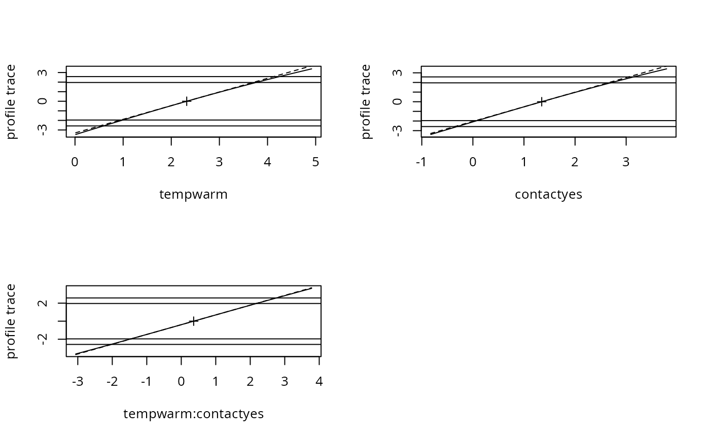
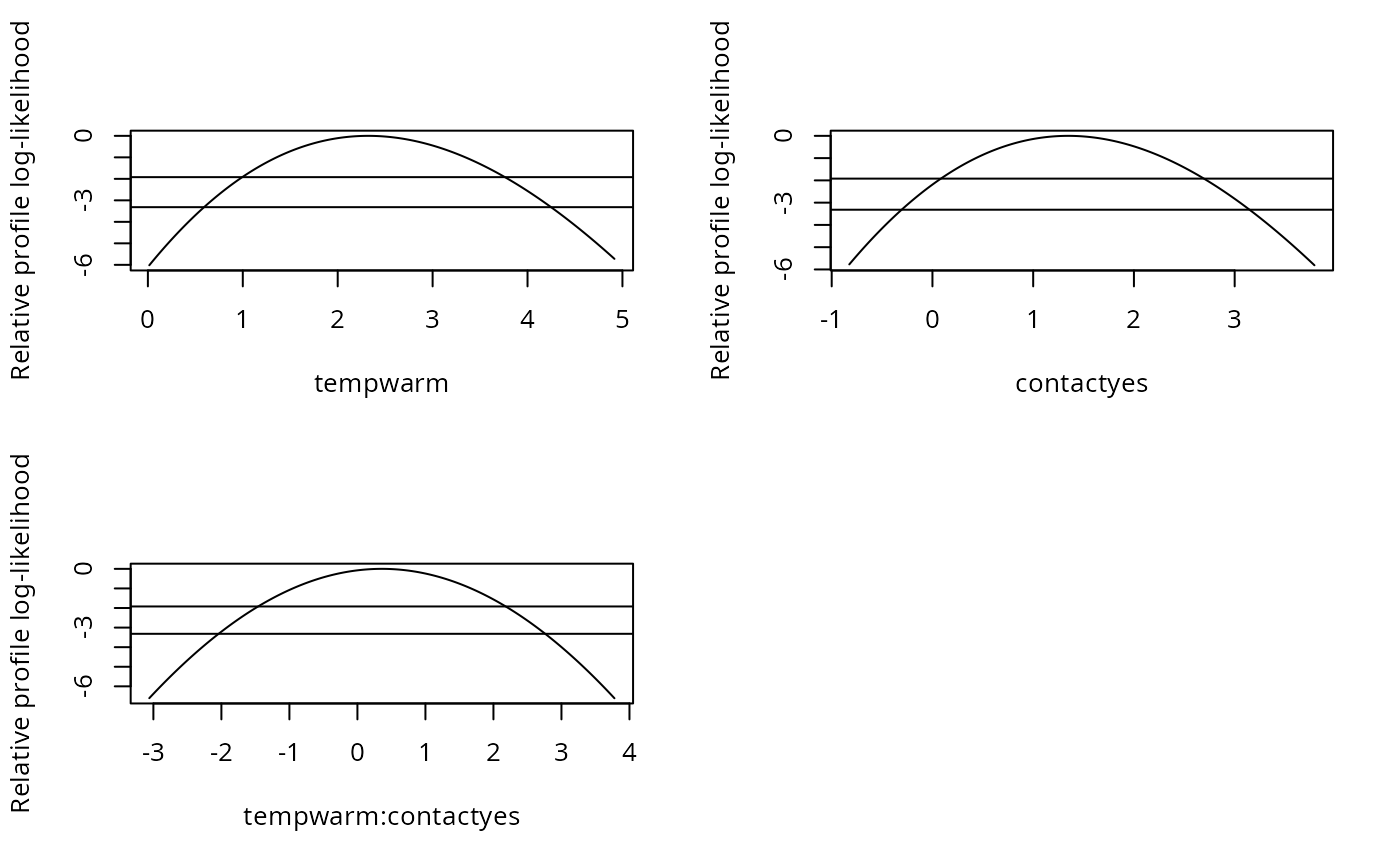
## plotting the profiles:
par(mfrow = c(2, 2))
plot(pr1, root = TRUE) ## check for linearity
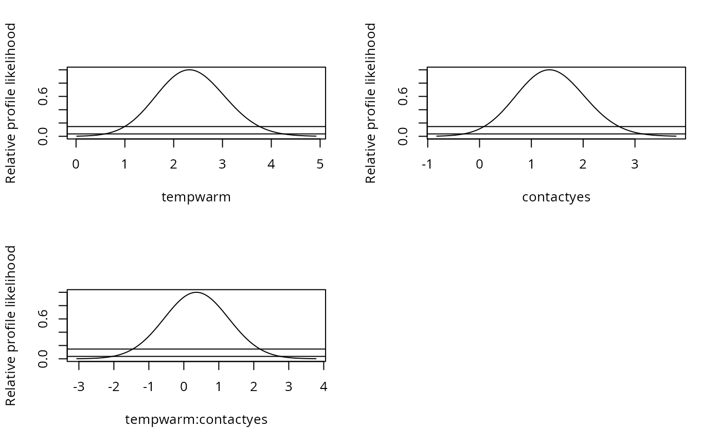
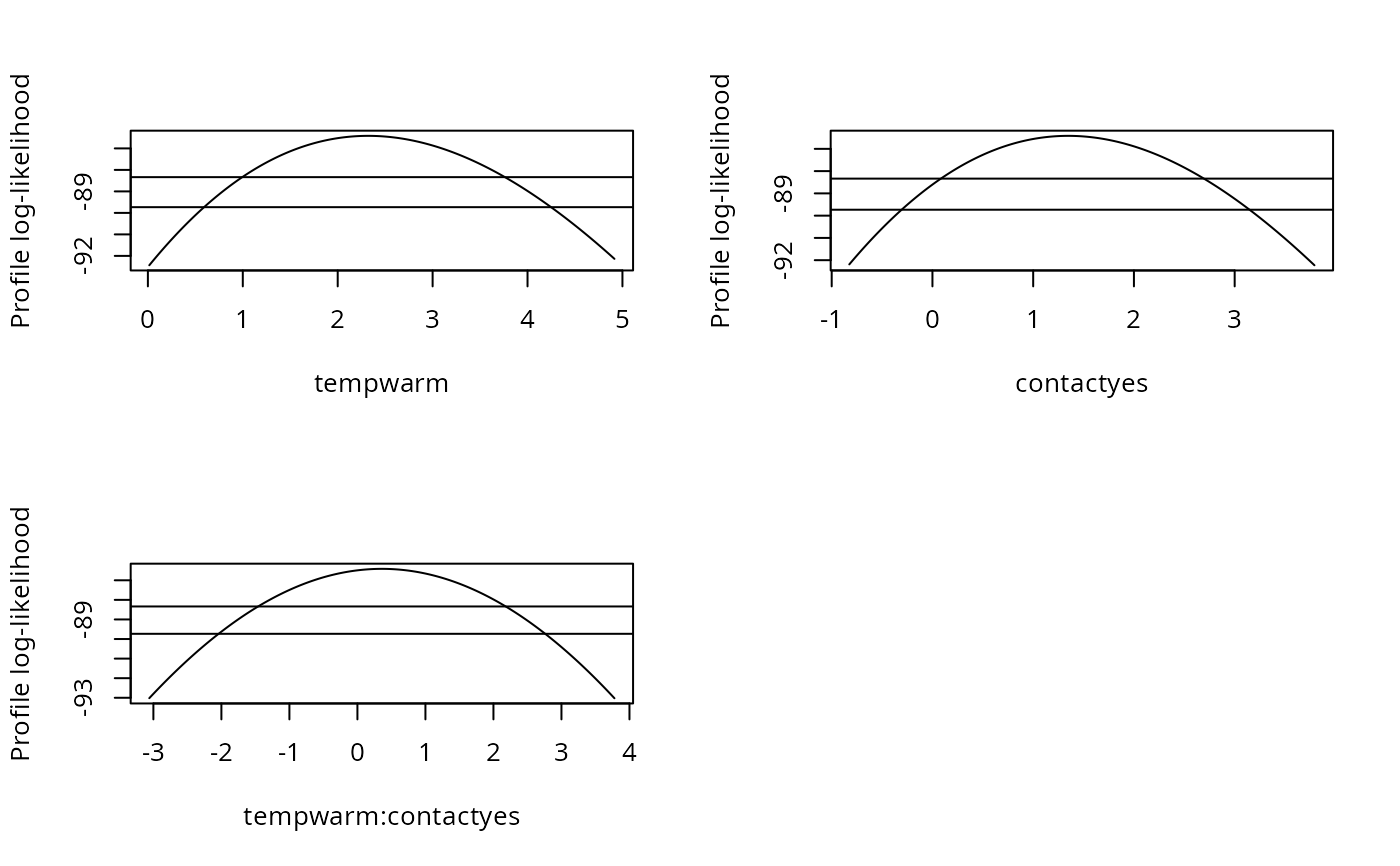
par(mfrow = c(2, 2))
 plot(pr1)
par(mfrow = c(2, 2))
plot(pr1)
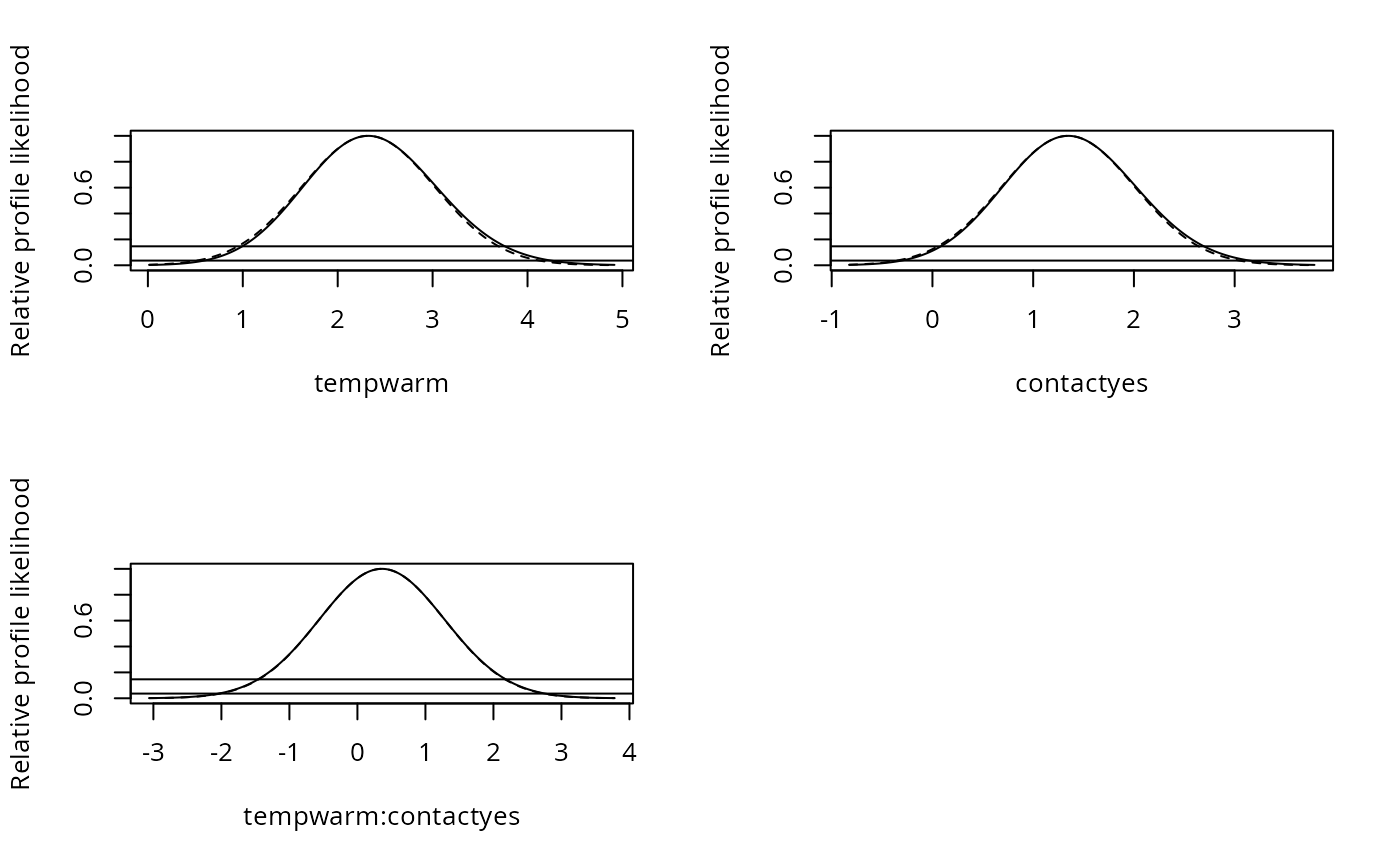
par(mfrow = c(2, 2))
 plot(pr1, approx = TRUE)
par(mfrow = c(2, 2))
plot(pr1, approx = TRUE)
par(mfrow = c(2, 2))
 plot(pr1, Log = TRUE)
par(mfrow = c(2, 2))
plot(pr1, Log = TRUE)
par(mfrow = c(2, 2))
 plot(pr1, Log = TRUE, relative = FALSE)
## other link functions:
fm4.lgt <- update(fm1, link = "logit") ## default
fm4.prt <- update(fm1, link = "probit")
fm4.ll <- update(fm1, link = "loglog")
fm4.cll <- update(fm1, link = "cloglog")
fm4.cct <- update(fm1, link = "cauchit")
anova(fm4.lgt, fm4.prt, fm4.ll, fm4.cll, fm4.cct)
#> Likelihood ratio tests of cumulative link models:
#>
#> formula: link: threshold:
#> fm4.lgt rating ~ temp * contact logit flexible
#> fm4.prt rating ~ temp * contact probit flexible
#> fm4.ll rating ~ temp * contact loglog flexible
#> fm4.cll rating ~ temp * contact cloglog flexible
#> fm4.cct rating ~ temp * contact cauchit flexible
#>
#> no.par AIC logLik LR.stat df Pr(>Chisq)
#> fm4.lgt 7 186.83 -86.416
#> fm4.prt 7 185.45 -85.723 1.3864 0
#> fm4.ll 7 189.14 -87.569 -3.6923 0
#> fm4.cll 7 187.22 -86.610 1.9175 0
#> fm4.cct 7 198.05 -92.027 -10.8323 0
## structured thresholds:
fm5 <- update(fm1, threshold = "symmetric")
fm6 <- update(fm1, threshold = "equidistant")
anova(fm1, fm5, fm6)
#> Likelihood ratio tests of cumulative link models:
#>
#> formula: link: threshold:
#> fm6 rating ~ temp * contact logit equidistant
#> fm5 rating ~ temp * contact logit symmetric
#> fm1 rating ~ temp * contact logit flexible
#>
#> no.par AIC logLik LR.stat df Pr(>Chisq)
#> fm6 5 185.14 -87.570
#> fm5 6 187.05 -87.527 0.0864 1 0.7688
#> fm1 7 186.83 -86.416 2.2220 1 0.1361
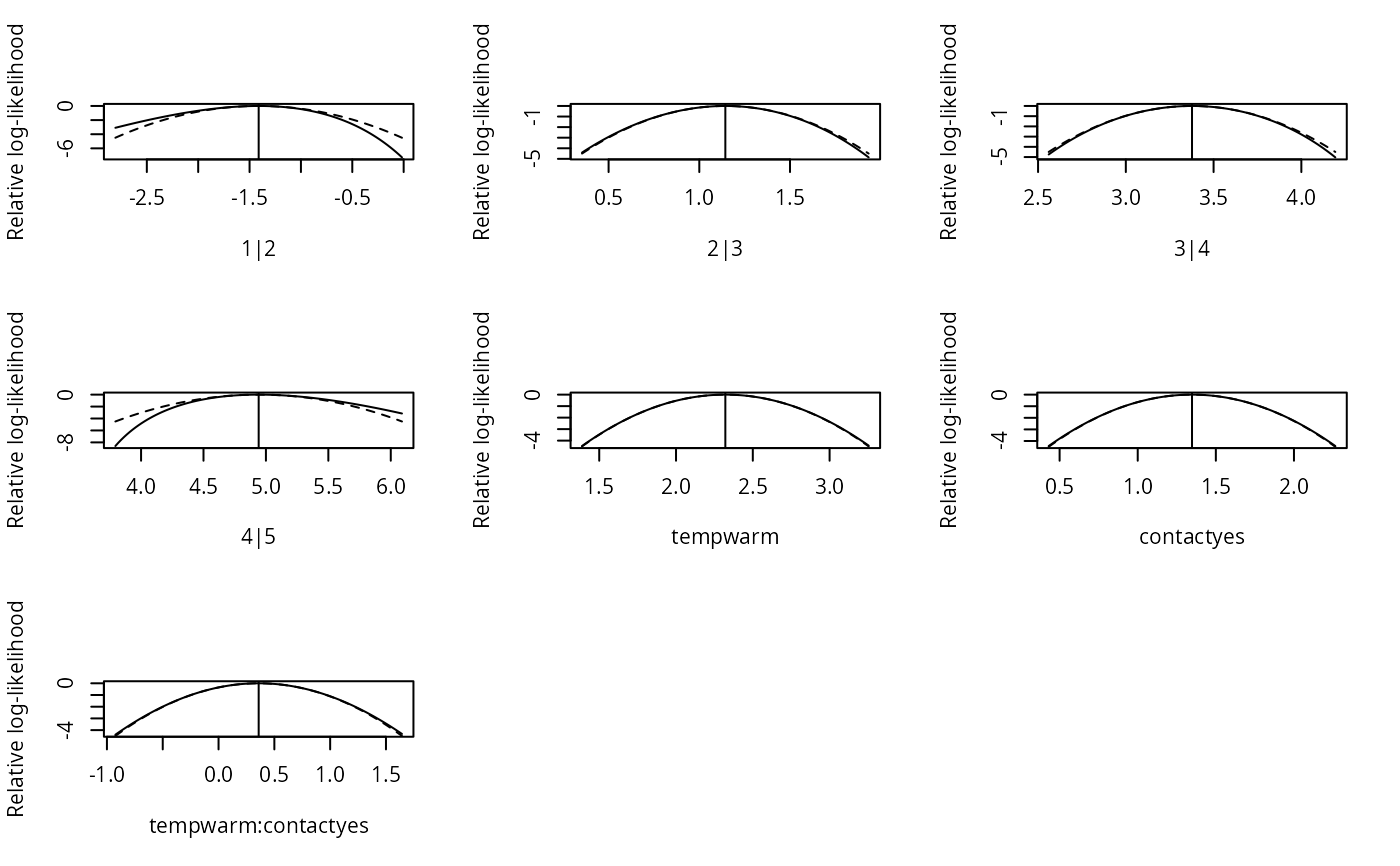
## the slice methods:
slice.fm1 <- slice(fm1)
par(mfrow = c(3, 3))
plot(pr1, Log = TRUE, relative = FALSE)
## other link functions:
fm4.lgt <- update(fm1, link = "logit") ## default
fm4.prt <- update(fm1, link = "probit")
fm4.ll <- update(fm1, link = "loglog")
fm4.cll <- update(fm1, link = "cloglog")
fm4.cct <- update(fm1, link = "cauchit")
anova(fm4.lgt, fm4.prt, fm4.ll, fm4.cll, fm4.cct)
#> Likelihood ratio tests of cumulative link models:
#>
#> formula: link: threshold:
#> fm4.lgt rating ~ temp * contact logit flexible
#> fm4.prt rating ~ temp * contact probit flexible
#> fm4.ll rating ~ temp * contact loglog flexible
#> fm4.cll rating ~ temp * contact cloglog flexible
#> fm4.cct rating ~ temp * contact cauchit flexible
#>
#> no.par AIC logLik LR.stat df Pr(>Chisq)
#> fm4.lgt 7 186.83 -86.416
#> fm4.prt 7 185.45 -85.723 1.3864 0
#> fm4.ll 7 189.14 -87.569 -3.6923 0
#> fm4.cll 7 187.22 -86.610 1.9175 0
#> fm4.cct 7 198.05 -92.027 -10.8323 0
## structured thresholds:
fm5 <- update(fm1, threshold = "symmetric")
fm6 <- update(fm1, threshold = "equidistant")
anova(fm1, fm5, fm6)
#> Likelihood ratio tests of cumulative link models:
#>
#> formula: link: threshold:
#> fm6 rating ~ temp * contact logit equidistant
#> fm5 rating ~ temp * contact logit symmetric
#> fm1 rating ~ temp * contact logit flexible
#>
#> no.par AIC logLik LR.stat df Pr(>Chisq)
#> fm6 5 185.14 -87.570
#> fm5 6 187.05 -87.527 0.0864 1 0.7688
#> fm1 7 186.83 -86.416 2.2220 1 0.1361
## the slice methods:
slice.fm1 <- slice(fm1)
par(mfrow = c(3, 3))
 plot(slice.fm1)
## see more at '?slice.clm'
## Another example:
fm.soup <- clm(SURENESS ~ PRODID, data = soup)
summary(fm.soup)
#> formula: SURENESS ~ PRODID
#> data: soup
#>
#> link threshold nobs logLik AIC niter max.grad cond.H
#> logit flexible 1847 -2677.27 5374.54 6(1) 7.39e-13 2.3e+02
#>
#> Coefficients:
#> Estimate Std. Error z value Pr(>|z|)
#> PRODID2 0.8925 0.1184 7.540 4.70e-14 ***
#> PRODID3 1.4477 0.1663 8.706 < 2e-16 ***
#> PRODID4 0.8325 0.1532 5.433 5.55e-08 ***
#> PRODID5 1.3109 0.1630 8.042 8.85e-16 ***
#> PRODID6 1.6010 0.1690 9.475 < 2e-16 ***
#> ---
#> Signif. codes: 0 ‘***’ 0.001 ‘**’ 0.01 ‘*’ 0.05 ‘.’ 0.1 ‘ ’ 1
#>
#> Threshold coefficients:
#> Estimate Std. Error z value
#> 1|2 -1.41244 0.08184 -17.258
#> 2|3 -0.42924 0.06972 -6.157
#> 3|4 -0.10340 0.06891 -1.500
#> 4|5 0.15121 0.06906 2.189
#> 5|6 0.82121 0.07201 11.404
if(require(MASS)) { ## dropterm, addterm, stepAIC, housing
fm1 <- clm(rating ~ temp * contact, data = wine)
dropterm(fm1, test = "Chi")
addterm(fm1, ~.+judge, test = "Chi")
fm3 <- stepAIC(fm1)
summary(fm3)
## Example from MASS::polr:
fm1 <- clm(Sat ~ Infl + Type + Cont, weights = Freq, data = housing)
summary(fm1)
}
#> Start: AIC=186.83
#> rating ~ temp * contact
#>
#> Df AIC
#> - temp:contact 1 184.98
#> <none> 186.83
#>
#> Step: AIC=184.98
#> rating ~ temp + contact
#>
#> Df AIC
#> <none> 184.98
#> - contact 1 194.03
#> - temp 1 209.91
#> formula: Sat ~ Infl + Type + Cont
#> data: housing
#>
#> link threshold nobs logLik AIC niter max.grad cond.H
#> logit flexible 1681 -1739.57 3495.15 4(0) 6.60e-09 4.7e+01
#>
#> Coefficients:
#> Estimate Std. Error z value Pr(>|z|)
#> InflMedium 0.56639 0.10465 5.412 6.23e-08 ***
#> InflHigh 1.28882 0.12716 10.136 < 2e-16 ***
#> TypeApartment -0.57235 0.11924 -4.800 1.59e-06 ***
#> TypeAtrium -0.36619 0.15517 -2.360 0.018282 *
#> TypeTerrace -1.09101 0.15149 -7.202 5.93e-13 ***
#> ContHigh 0.36028 0.09554 3.771 0.000162 ***
#> ---
#> Signif. codes: 0 ‘***’ 0.001 ‘**’ 0.01 ‘*’ 0.05 ‘.’ 0.1 ‘ ’ 1
#>
#> Threshold coefficients:
#> Estimate Std. Error z value
#> Low|Medium -0.4961 0.1248 -3.974
#> Medium|High 0.6907 0.1255 5.505
plot(slice.fm1)
## see more at '?slice.clm'
## Another example:
fm.soup <- clm(SURENESS ~ PRODID, data = soup)
summary(fm.soup)
#> formula: SURENESS ~ PRODID
#> data: soup
#>
#> link threshold nobs logLik AIC niter max.grad cond.H
#> logit flexible 1847 -2677.27 5374.54 6(1) 7.39e-13 2.3e+02
#>
#> Coefficients:
#> Estimate Std. Error z value Pr(>|z|)
#> PRODID2 0.8925 0.1184 7.540 4.70e-14 ***
#> PRODID3 1.4477 0.1663 8.706 < 2e-16 ***
#> PRODID4 0.8325 0.1532 5.433 5.55e-08 ***
#> PRODID5 1.3109 0.1630 8.042 8.85e-16 ***
#> PRODID6 1.6010 0.1690 9.475 < 2e-16 ***
#> ---
#> Signif. codes: 0 ‘***’ 0.001 ‘**’ 0.01 ‘*’ 0.05 ‘.’ 0.1 ‘ ’ 1
#>
#> Threshold coefficients:
#> Estimate Std. Error z value
#> 1|2 -1.41244 0.08184 -17.258
#> 2|3 -0.42924 0.06972 -6.157
#> 3|4 -0.10340 0.06891 -1.500
#> 4|5 0.15121 0.06906 2.189
#> 5|6 0.82121 0.07201 11.404
if(require(MASS)) { ## dropterm, addterm, stepAIC, housing
fm1 <- clm(rating ~ temp * contact, data = wine)
dropterm(fm1, test = "Chi")
addterm(fm1, ~.+judge, test = "Chi")
fm3 <- stepAIC(fm1)
summary(fm3)
## Example from MASS::polr:
fm1 <- clm(Sat ~ Infl + Type + Cont, weights = Freq, data = housing)
summary(fm1)
}
#> Start: AIC=186.83
#> rating ~ temp * contact
#>
#> Df AIC
#> - temp:contact 1 184.98
#> <none> 186.83
#>
#> Step: AIC=184.98
#> rating ~ temp + contact
#>
#> Df AIC
#> <none> 184.98
#> - contact 1 194.03
#> - temp 1 209.91
#> formula: Sat ~ Infl + Type + Cont
#> data: housing
#>
#> link threshold nobs logLik AIC niter max.grad cond.H
#> logit flexible 1681 -1739.57 3495.15 4(0) 6.60e-09 4.7e+01
#>
#> Coefficients:
#> Estimate Std. Error z value Pr(>|z|)
#> InflMedium 0.56639 0.10465 5.412 6.23e-08 ***
#> InflHigh 1.28882 0.12716 10.136 < 2e-16 ***
#> TypeApartment -0.57235 0.11924 -4.800 1.59e-06 ***
#> TypeAtrium -0.36619 0.15517 -2.360 0.018282 *
#> TypeTerrace -1.09101 0.15149 -7.202 5.93e-13 ***
#> ContHigh 0.36028 0.09554 3.771 0.000162 ***
#> ---
#> Signif. codes: 0 ‘***’ 0.001 ‘**’ 0.01 ‘*’ 0.05 ‘.’ 0.1 ‘ ’ 1
#>
#> Threshold coefficients:
#> Estimate Std. Error z value
#> Low|Medium -0.4961 0.1248 -3.974
#> Medium|High 0.6907 0.1255 5.505