Getting Started with Narnia
Nicholas Tierney
2017-07-25
Introduction
Missing values are ubiquitous in data and need to be carefully explored and handled in the initial stages of analysis. In this vignette we describe the tools in the package narnia for exploring missing data structures with minimal deviation from the common workflows of ggplot and tidy data [@Wickham2014; @Wickham2009].
Sometimes researchers or analysts will introduce or describe a mechanism for missingness. For example, they might explain that data from a weather station might has a malfunction when there are extreme weather events, and does not record temperature data when gusts speeds are high. This seems like a nice simple, logical explanation. However, like all good explanations, this one is simple, but the process to get there, probably was not, and likely involved more time than you would have liked developing exploratory data analyses and models.
So when someone presents a really obvious plot like this, with a nice sensible explanation, the initial thought might be:
They worked it out themselves so quickly, so easy!
As if they somehow accidentally solved the problem, it was so easy. They couldn’t not solve it. However, I think that if you manage to get that on the first go, that is more like turning around and throwing a rock into a lake and it landing in a cup in a boat. Unlikely.
With that thought in mind, this vignette aims to work with the following three questions, using the tools developed in narnia and another package, visdat. Namely, how do we:
- Start looking at missing data?
- Explore missingness mechanisms?
- Model missingness?
How do we start looking at missing data?
When you start with a dataset, you might do something where you look at the general summary, using functions such as:
summary()str()-
skimr::skim, or dplyr::glimpse()
These works really well when you’ve got a small amount of data, but when you have more data, you are generally limited by how much you can read.
So before you start looking at missing data, you’ll need to look at the data, but what does that even mean?
The package visdat helps you get a handle on this. visdat provides a visualisation of an entire data frame at once, and was heavily inspired by csv-fingerprint, and the missingness map functions from packages like Amelia::missmap.
There are two main functions in the visdat package:
-
vis_dat, and vis_miss
vis_dat
library(visdat)
vis_dat(airquality)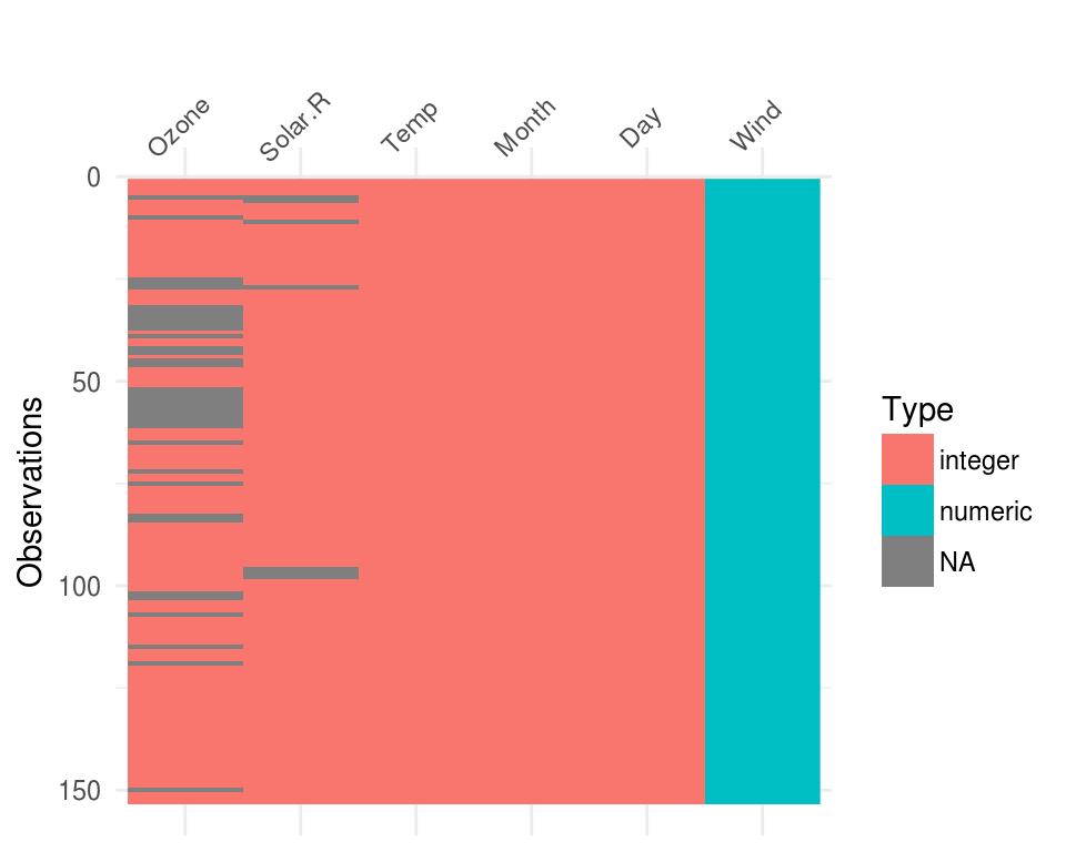
These visualise the whole dataframe at once, and provide some useful information about whether the data is missing or not. It also provides information about the class of the data input into R.
The function vis_miss provides a summary of whether the data is all present, and also provides small summaries in each column as to the amount of missings in each of the columns.
vis_miss
vis_miss(airquality)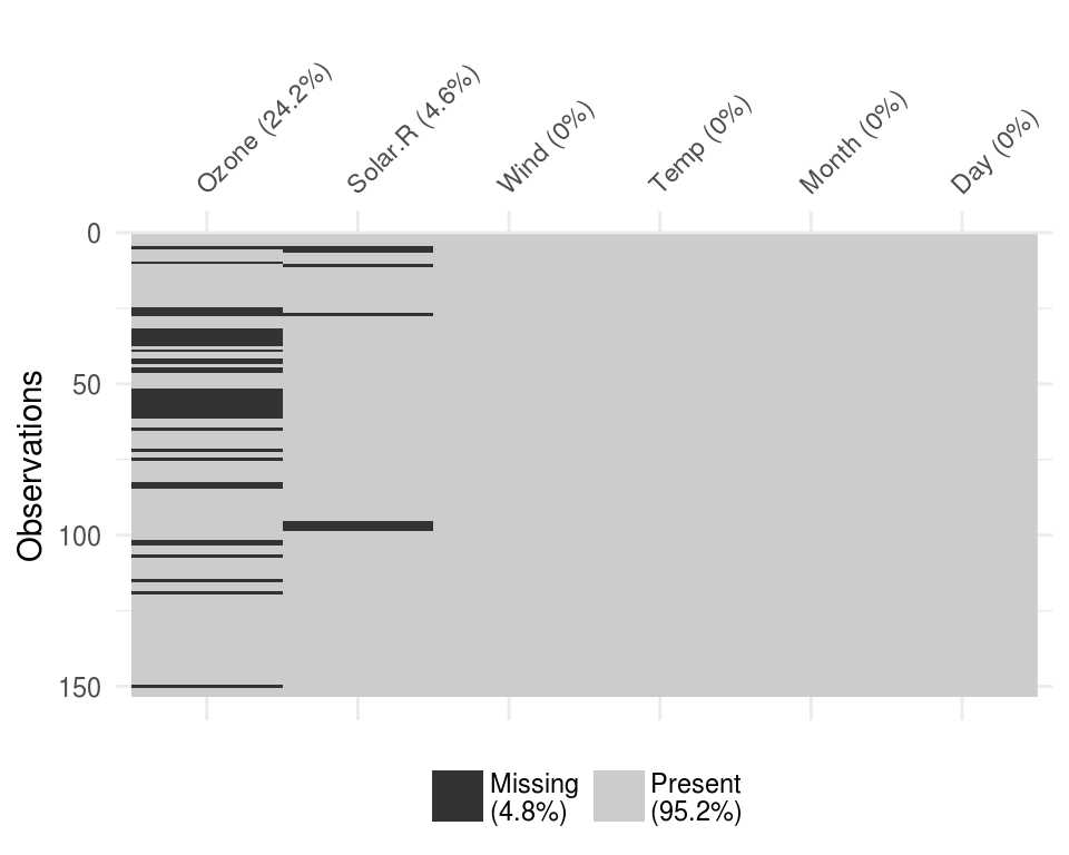
To read more about the functions available in visdat see the vignette “Using visdat”
Exploring missingness relationships
We can identify key variables that are missing
For further exploration, we need to explore the relationship amongst the variables in this data:
- Ozone,
- Solar.R
- Wind
- Temp
- Month
- Day
This process of visualising the data as a heatmap allows you identify what is missing and where. For here though, are interested in exploring these missingness relationships.
Typically, when exploring this data, you might want to explore the variables Solar.R and Ozone, and do something like this:
library(ggplot2)
ggplot(airquality,
       aes(x = Solar.R,
           y = Ozone)) +
  geom_point()
## Warning: Removed 42 rows containing missing values (geom_point).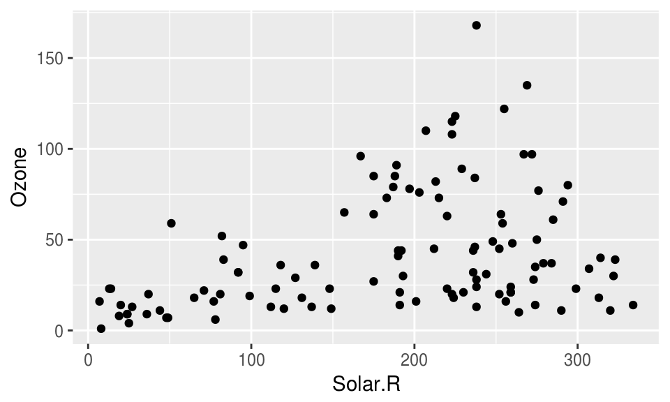
The problem with this is that ggplot does not handle missings be default, and removes the missing values. This makes them hard to explore.
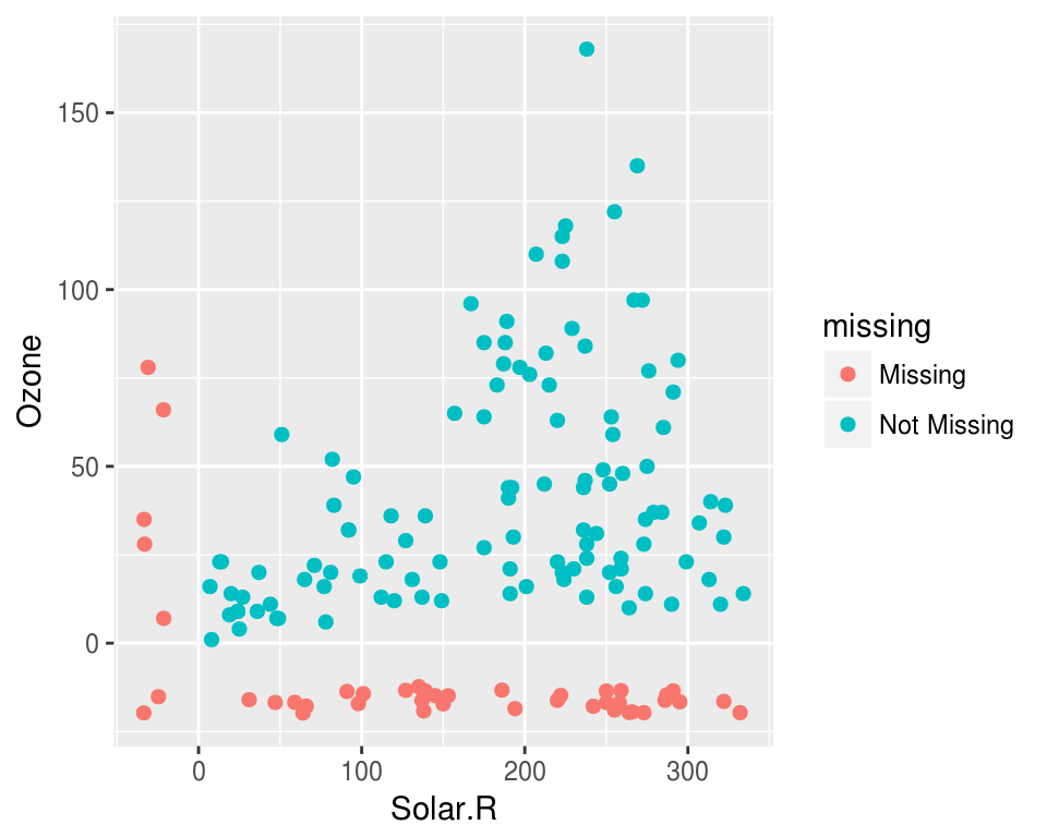
Visualising missing data might sound a little strange - how do you visualise something that is not there? One approach to visualising missing data comes from ggobi and manet, where we replace “NA” values with values 10% lower than the minimum value in that variable. This is provided with the geom_miss_point() ggplot2 geom, which we can illustrate by exploring the relationship between Ozone and Solar radiation from the airquality dataset.
ggplot(airquality,
       aes(x = Solar.R,
           y = Ozone)) +
  geom_point()
## Warning: Removed 42 rows containing missing values (geom_point).library(narnia)
ggplot(airquality,
aes(x = Solar.R,
y = Ozone)) +
geom_miss_point()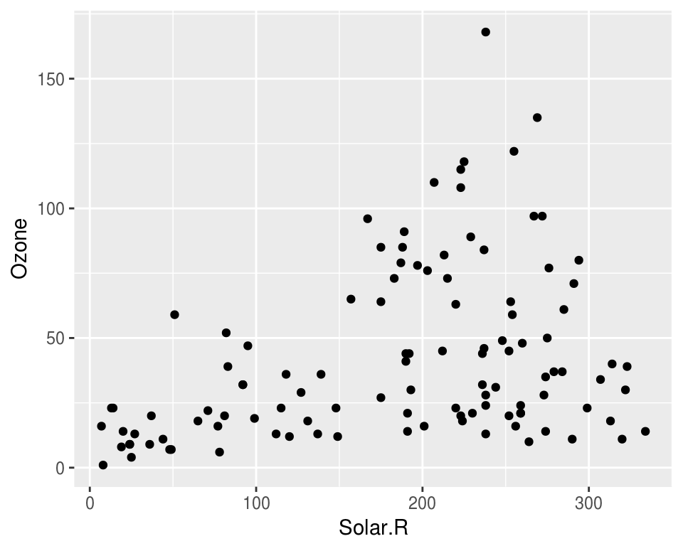
Facets!
ggplot(airquality,
       aes(x = Solar.R,
           y = Ozone)) +
  geom_miss_point() +
  facet_wrap(~Month)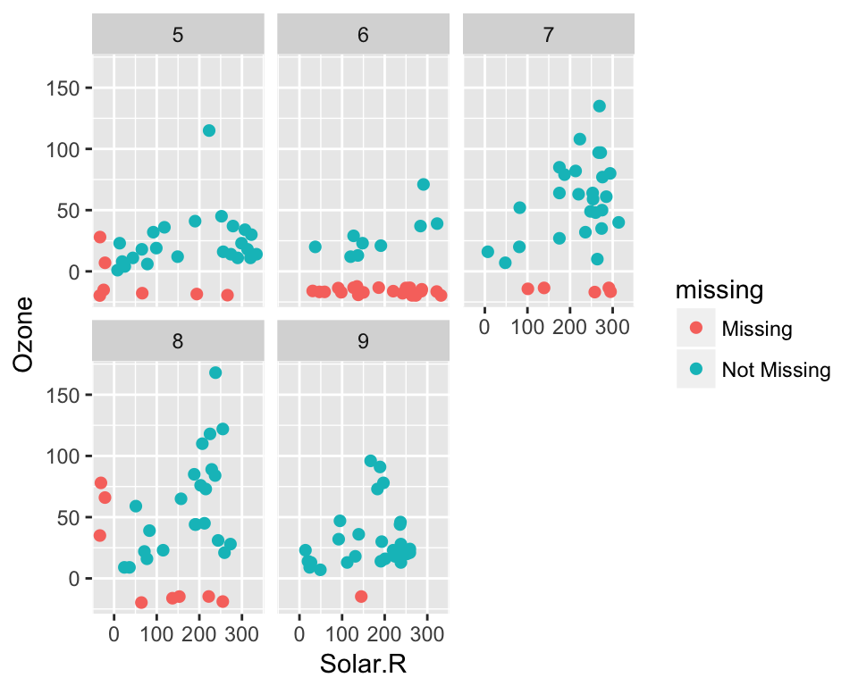
Themes!
ggplot(airquality,
       aes(x = Solar.R,
           y = Ozone)) +
  geom_miss_point() +
  facet_wrap(~Month) +
  theme_dark()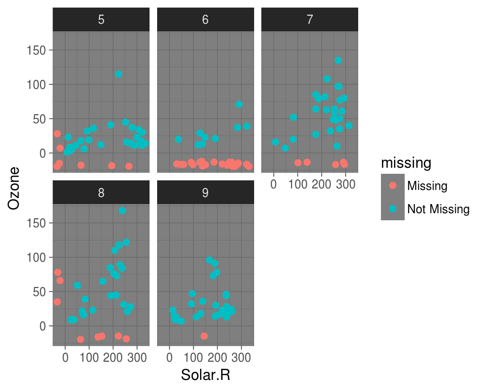
Visualising missings in variables
Another approach to visualising the missings in a dataset is to use the gg_miss_var plot:
gg_miss_var(airquality)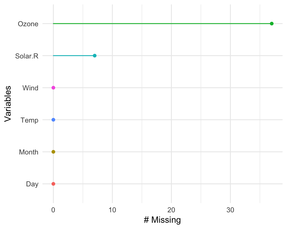
This creates a ggplot2 object with the number of missing values for each variable, ordered from most missing to least missing. Under the hood, this is powered using miss_var_summary(), described later.
The plots created with the gg_miss family all have a basic theme, but you can customise them, just like usual ggplot objects. If you call any ggplot customisation functions with a gg_miss object, the default args will be overridden.
gg_miss_var(airquality) + theme_bw() 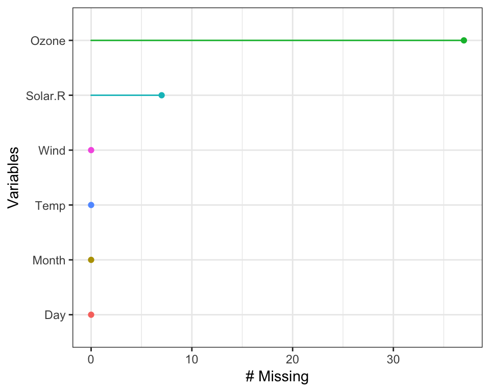
gg_miss_var(airquality) + labs(y = "Look at all the missing ones")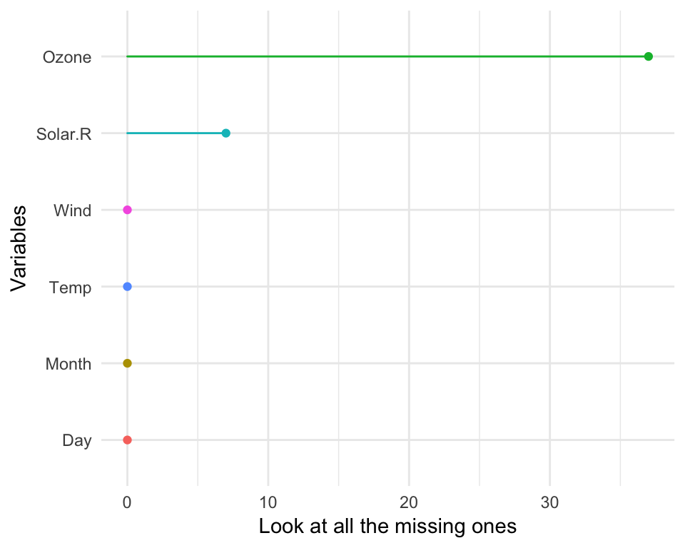
shadow matrix: A tidy way of representing missing values
Representing missing data structure is achieved using the shadow matrix, introduced in Swayne and Buja. The shadow matrix is the same dimension as the data, and consists of binary indicators of missingness of data values, where missing is represented as “NA”, and not missing is represented as “!NA”. Although these may be represented as 1 and 0, respectively. This representation can be seen in the figure below, adding the suffix “_NA" to the variables. This structure can also be extended to allow for additional factor levels to be created. For example 0 indicates data presence, 1 indicates missing values, 2 indicates imputed value, and 3 might indicate a particular type or class of missingness, where reasons for missingness might be known or inferred. The data matrix can also be augmented to include the shadow matrix, which facilitates visualisation of univariate and bivariate missing data visualisations. Another format is to display it in long form, which facilitates heatmap style visualisations. This approach can be very helpful for giving an overview of which variables contain the most missingness. Methods can also be applied to rearrange rows and columns to find clusters, and identify other interesting features of the data that may have previously been hidden or unclear.
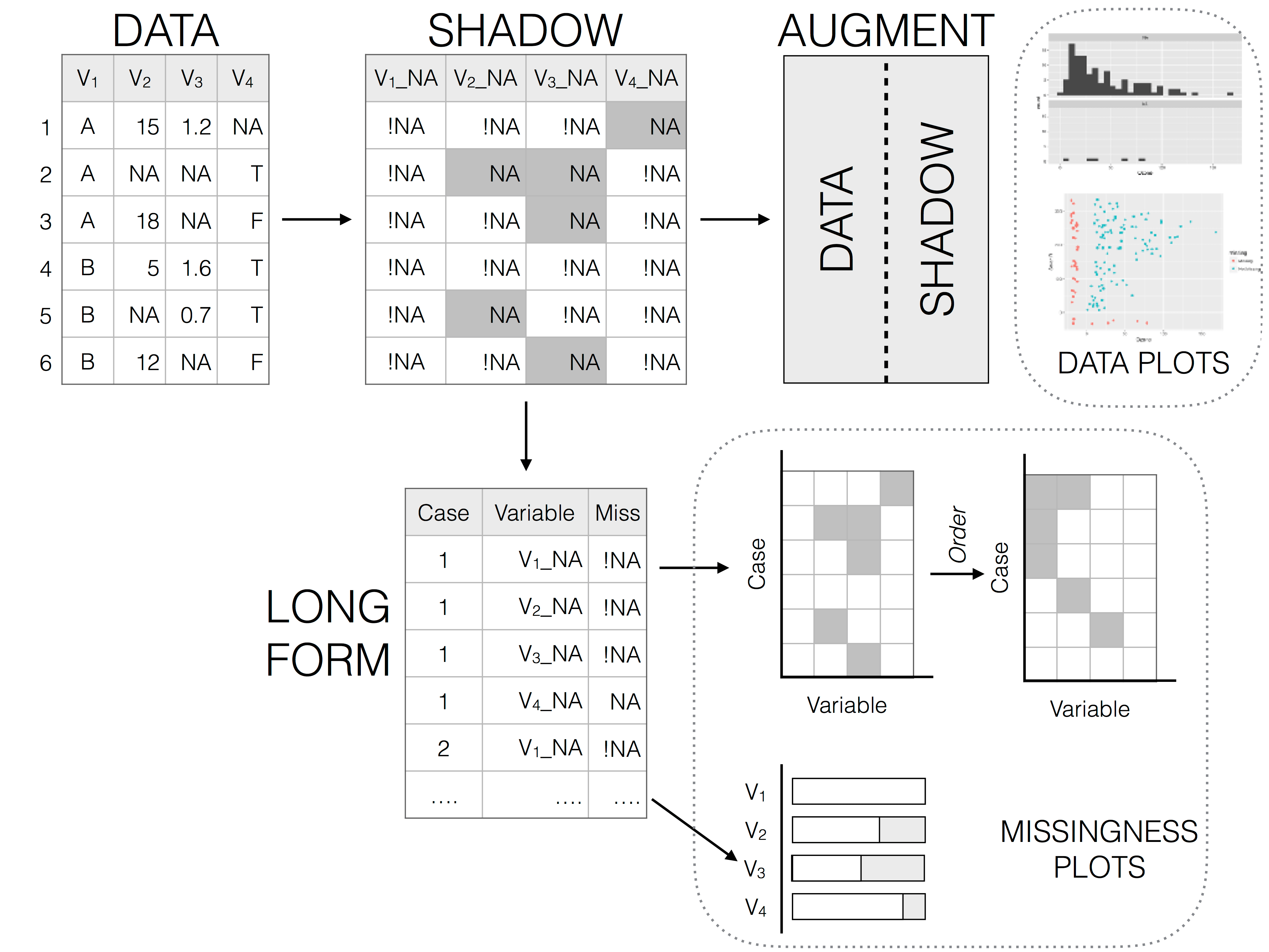
Illustration of data structures for facilitating visualisation of missings and not missings
The shadow functions provide a way to keep track of missing values. The as_shadow function creates a dataframe with the same set of columns, but with the column names added a suffix _NA
as_shadow(airquality)## # A tibble: 153 x 6
## Ozone_NA Solar.R_NA Wind_NA Temp_NA Month_NA Day_NA
## <fctr> <fctr> <fctr> <fctr> <fctr> <fctr>
## 1 !NA !NA !NA !NA !NA !NA
## 2 !NA !NA !NA !NA !NA !NA
## 3 !NA !NA !NA !NA !NA !NA
## 4 !NA !NA !NA !NA !NA !NA
## 5 NA NA !NA !NA !NA !NA
## 6 !NA NA !NA !NA !NA !NA
## 7 !NA !NA !NA !NA !NA !NA
## 8 !NA !NA !NA !NA !NA !NA
## 9 !NA !NA !NA !NA !NA !NA
## 10 NA !NA !NA !NA !NA !NA
## # ... with 143 more rowsThe bind_shadow argument attaches a shadow to the current dataframe
aq_shadow <- bind_shadow(airquality)

library(dplyr)
##
## Attaching package: 'dplyr'## The following objects are masked from 'package:stats':
##
## filter, lag## The following objects are masked from 'package:base':
##
## intersect, setdiff, setequal, unionglimpse(aq_shadow)## Observations: 153
## Variables: 12
## $ Ozone <int> 41, 36, 12, 18, NA, 28, 23, 19, 8, NA, 7, 16, 11, 1...
## $ Solar.R <int> 190, 118, 149, 313, NA, NA, 299, 99, 19, 194, NA, 2...
## $ Wind <dbl> 7.4, 8.0, 12.6, 11.5, 14.3, 14.9, 8.6, 13.8, 20.1, ...
## $ Temp <int> 67, 72, 74, 62, 56, 66, 65, 59, 61, 69, 74, 69, 66,...
## $ Month <int> 5, 5, 5, 5, 5, 5, 5, 5, 5, 5, 5, 5, 5, 5, 5, 5, 5, ...
## $ Day <int> 1, 2, 3, 4, 5, 6, 7, 8, 9, 10, 11, 12, 13, 14, 15, ...
## $ Ozone_NA <fctr> !NA, !NA, !NA, !NA, NA, !NA, !NA, !NA, !NA, NA, !N...
## $ Solar.R_NA <fctr> !NA, !NA, !NA, !NA, NA, NA, !NA, !NA, !NA, !NA, NA...
## $ Wind_NA <fctr> !NA, !NA, !NA, !NA, !NA, !NA, !NA, !NA, !NA, !NA, ...
## $ Temp_NA <fctr> !NA, !NA, !NA, !NA, !NA, !NA, !NA, !NA, !NA, !NA, ...
## $ Month_NA <fctr> !NA, !NA, !NA, !NA, !NA, !NA, !NA, !NA, !NA, !NA, ...
## $ Day_NA <fctr> !NA, !NA, !NA, !NA, !NA, !NA, !NA, !NA, !NA, !NA, ...Doing this provides a consistent syntax for referring to variables with missing values.
bind_shadow() also provides a useful pattern to explore missing values by grouping by the missing/complete of one variable and looking at the mean and other summary values. Below we show the mean, sd, variance, and min and max values of Solar.R for when Ozone is present, and when it is missing.
airquality %>%
  bind_shadow() %>%
  group_by(Ozone_NA) %>%
  summarise_at(.vars = "Solar.R",
               .funs = c("mean", "sd", "var", "min", "max"),
               na.rm = TRUE)
## # A tibble: 2 x 6
## Ozone_NA mean sd var min max
## <fctr> <dbl> <dbl> <dbl> <dbl> <dbl>
## 1 !NA 184.8018 91.15230 8308.742 7 334
## 2 NA 189.5143 87.69478 7690.375 31 332Below, we can plot the distribution of Temperature, plotting for values of temperature when Ozone is missing, and when it is not missing.
ggplot(aq_shadow,
       aes(x = Temp,
           colour = Ozone_NA)) +
  geom_density()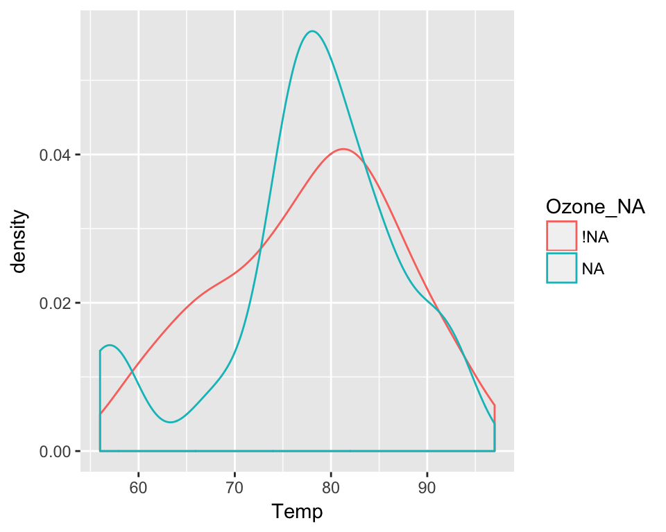
Binding the shadow here also has great benefits when combined with imputation.
Visualising imputed values
Using the easy-to-use simputation package, we impute values for Ozone, then visualise the data:
library(simputation)
library(dplyr)

airquality %>%
  impute_lm(Ozone ~ Temp + Wind) %>%
  ggplot(aes(x = Temp,
             y = Ozone)) +
  geom_point()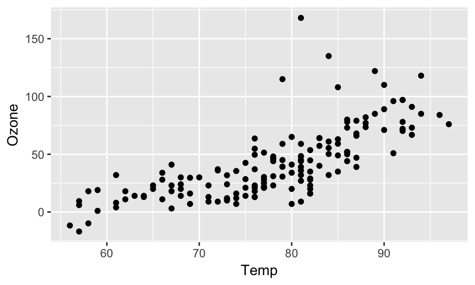
Note that we no longer get any errors regarding missing observations - because they are all imputed! But this comes at a cost: we also no longer have information about where the imputations are - they are now sort of invisible.
Using the shadow matrix to keep track of where the missings are, you can actually keep track of the imputations, by colouring by what was previously missing in Ozone.
aq_shadow %>%
  impute_lm(Ozone ~ Temp + Wind) %>%
  ggplot(aes(x = Temp,
             y = Ozone,
             colour = Ozone_NA)) +
  geom_point()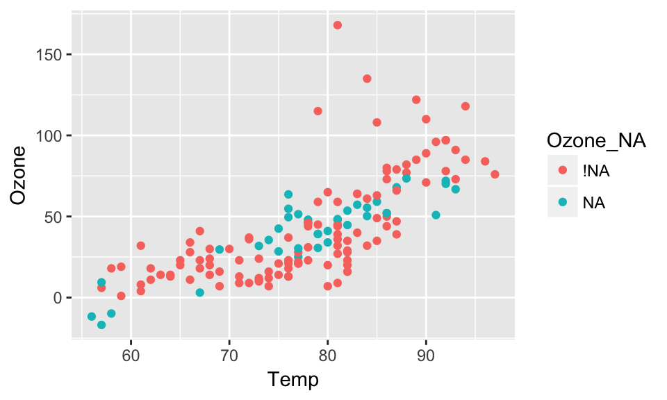
Numerical summaries of missing values
narnia also provide numerical summaries for missing data. Two convenient counters of complete values and missings are n_miss and n_complete. These work on both dataframes and vectors, similar to dplyr::n_distinct
dplyr::n_distinct(airquality)## [1] 153dplyr::n_distinct(airquality$Ozone)## [1] 68n_miss(airquality)## [1] 44n_miss(airquality$Ozone)## [1] 37n_complete(airquality)## [1] 874n_complete(airquality$Ozone)## [1] 116The syntax for the other numerical sumamries in narnia are miss_, and then case, var, or df, and then summary or table. There are also some summary functions for ts objects that are being worked on, which currently have miss_ts_run and miss_ts_summary functions.
To demonstrate, below are the miss_case_* family of functions.
miss_case_pct returns a numeric value describing the percent of missing values in the dataframe.
miss_case_pct(airquality)## [1] 27.45098miss_case_summary returns a numeric value that describes the number of missings in a given case (aka row), the percent of missings in that row.
miss_case_summary(airquality)## # A tibble: 153 x 3
## case n_miss pct_miss
## <int> <int> <dbl>
## 1 1 0 0.00000
## 2 2 0 0.00000
## 3 3 0 0.00000
## 4 4 0 0.00000
## 5 5 2 33.33333
## 6 6 1 16.66667
## 7 7 0 0.00000
## 8 8 0 0.00000
## 9 9 0 0.00000
## 10 10 1 16.66667
## # ... with 143 more rowsmiss_case_table tabulates the number of missing values in a case / row. Below, this shows the number of missings in a case:
- There are 111 cases with 0 missings, which comprises about 72% of the data.
- There are then 40 cases with 1 missing, these make up 26% of the data.
- There are then 2 cases with 2 missing - these make up 1% of the data.
miss_case_table(airquality)## # A tibble: 3 x 3
## n_miss_in_case n_cases pct_miss
## <int> <int> <dbl>
## 1 0 111 72.54902
## 2 1 40 26.14379
## 3 2 2 1.30719There are then the miss_var_* family of functions.
Similar to miss_case_pct, miss_var_pct returns the percent of variables that contain a missing value.
miss_var_pct(airquality)## [1] 33.33333miss_var_summary then returns the number of missing values in a variable, and the percent missing in that variable.
miss_var_summary(airquality)## # A tibble: 6 x 3
## variable n_miss pct_miss
## <chr> <int> <dbl>
## 1 Ozone 37 24.183007
## 2 Solar.R 7 4.575163
## 3 Wind 0 0.000000
## 4 Temp 0 0.000000
## 5 Month 0 0.000000
## 6 Day 0 0.000000Finally, miss_var_table. This describes the number of missings in a variable.
- There are 4 variables with 0 missings, comprising 66.67% of variables in the dataset.
- There is 1 variable with 7 missings
- There is 1 variable with 37 missings
miss_var_table(airquality)## # A tibble: 3 x 3
## n_miss_in_var n_vars pct_miss
## <int> <int> <dbl>
## 1 0 4 66.66667
## 2 7 1 16.66667
## 3 37 1 16.66667There are also summary functions for exploring missings that occur over a particular span or period of the dataset, or the number of missings in a single run:
miss_var_run can be particularly useful in time series data, as it allows you to provide summaries for the number of missings or complete values in a single run. The function miss_var_run() provides a data.frame of the run length of missings and complete values. To explore this function we will use the built-in dataset, pedestrian, which contains hourly counts of pedestrians from four locations around Melbourne, Australia, from 2016.
To use miss_var_run, you specify the variable that you want to explore the runs of missingness for, in this case, hourly_counts:
miss_var_run(pedestrian,
             hourly_counts)
## # A tibble: 35 x 2
## run_length is_na
## <int> <chr>
## 1 6628 complete
## 2 1 missing
## 3 5250 complete
## 4 624 missing
## 5 3652 complete
## 6 1 missing
## 7 1290 complete
## 8 744 missing
## 9 7420 complete
## 10 1 missing
## # ... with 25 more rowsmiss_var_span() is used to determine the number of missings over a specified repeating span of rows in variable of a dataframe. Similar to miss_var_run, you specify the variable that you wish to explore, you then also specify the size of the span with the span_every argument.
miss_var_span(pedestrian,
              hourly_counts,
              span_every = 100)
## # A tibble: 377 x 5
## span_counter n_miss n_complete prop_miss prop_complete
## <int> <int> <dbl> <dbl> <dbl>
## 1 1 0 100 0 1
## 2 2 0 100 0 1
## 3 3 0 100 0 1
## 4 4 0 100 0 1
## 5 5 0 100 0 1
## 6 6 0 100 0 1
## 7 7 0 100 0 1
## 8 8 0 100 0 1
## 9 9 0 100 0 1
## 10 10 0 100 0 1
## # ... with 367 more rowsThe final question we proposed in this vignette was:
- Can we model missingness?
Sometimes it can be impractical to explore all of the variables that have missing data. One approach, however, is to model missing data using methods from Tierney et el. (2015).
Here, the approach is to predict the proportion of missingness in a given case, using all variables. There is a little helper function to add a column with the proportion of cases or rows missing - add_prop_miss. This created a column named “prop_miss”, which is the proportion of missing values in that row.
airquality %>%
  add_prop_miss() %>%
  head()
## # A tibble: 6 x 7
## Ozone Solar.R Wind Temp Month Day prop_miss_all
## <int> <int> <dbl> <int> <int> <int> <dbl>
## 1 41 190 7.4 67 5 1 0.0000000
## 2 36 118 8.0 72 5 2 0.0000000
## 3 12 149 12.6 74 5 3 0.0000000
## 4 18 313 11.5 62 5 4 0.0000000
## 5 NA NA 14.3 56 5 5 0.3333333
## 6 28 NA 14.9 66 5 6 0.1666667We can then use a model like decision trees to predict which variables and their values are important for predicting the proportion of missingness:
library(rpart)
library(rpart.plot)

airquality %>%
  add_prop_miss() %>%
  rpart(prop_miss_all ~ ., data = .) %>%
  prp(type = 4, extra = 101, prefix = "Prop. Miss = ")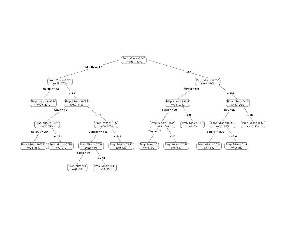
# library(visdat)
# vis_miss(messy_airquality)
Here we can see that this produces quite a complex tree - this can be pruned back and the depth of the decision tree controlled.
Summary
The tools in narnia help us identify where missingness is, while maintaining a tidy workflow. We care about these mechanisms or these patterns because they can help us understand potential mechanisms, such as equipment failures, and then identify possible solutions based upon this evidence.
Future development
- Continue making
narniaplay well withdplyrandtidyr. - Make
narniawork with big data tools likesparklyr, andsparklingwater. - Expand ggplot
geom_miss_*family. - Further develop methods for handling and visualising imputations, and multiple imputation.
Thank you
A huge thanks of course to Di Cook and Miles McBain for their assistance on this project, and its development. In particular, I thank Di for providing the large conceptual ideas of how to display missings, and the use of the shadow matrix. I also thank Miles for his instrumental work in getting stat_missing_point and geom_miss_point() working as they do now.
References
- MANET: http://www.rosuda.org/MANET/
- ggobi: http://www.ggobi.org/
- visdat: https://www.github.com/njtierney/visdat
- Tierney NJ, Harden FA, Harden MJ, Mengersen, KA, Using decision trees to understand structure in missing data BMJ Open 2015;5:e007450. doi: 10.1136/bmjopen-2014-007450