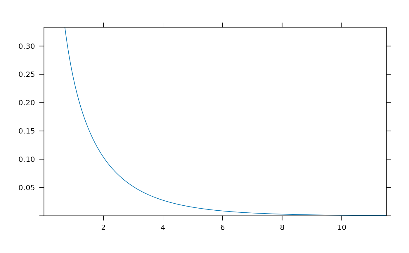
Plots of Discrete and Continuous Distributions

Provides a simple way to generate plots of pdfs, probability mass functions, cdfs, probability histograms, and normal-quantile plots for distributions known to R.

Usage

plotDist(
  dist,
  ...,
  xlim = NULL,
  ylim = NULL,
  add,
  under = FALSE,
  packets = NULL,
  rows = NULL,
  columns = NULL,
  kind = c("density", "cdf", "qq", "histogram"),
  xlab = "",
  ylab = "",
  breaks = NULL,
  type,
  resolution = 5000L,
  params = NULL
)

Arguments

dist: A string identifying the distribution. This should work with any distribution that has associated functions beginning with 'd', 'p', and 'q' (e.g, dnorm(), pnorm(), and qnorm()). dist should match the name of the distribution with the initial 'd', 'p', or 'q' removed.
...: other arguments passed along to lattice graphing routines
xlim: a numeric vector of length 2 or NULL, in which case the central 99.8 of the distribution is used.
ylim: a numeric vector of length 2 or NULL, in which case a heuristic is used to avoid chasing asymptotes in distributions like the F distributions with 1 numerator degree of freedom.
add: a logical indicating whether the plot should be added to the previous lattice plot. If missing, it will be set to match under.
under: a logical indicating whether adding should be done in a layer under or over the existing layers when add = TRUE.
packets, rows, columns: specification of which panels will be added to when add is TRUE. See latticeExtra::layer().
kind: one of "density", "cdf", "qq", or "histogram" (or prefix of any of these)
xlab, ylab: as per other lattice functions
breaks: a vector of break points for bins of histograms, as in histogram()
type: passed along to various lattice graphing functions
resolution: number of points to sample when generating the plots
params: a list containing parameters for the distribution. If NULL (the default), this list is created from elements of \dots that are either unnamed or have names among the formals of the appropriate distribution function. See the examples.

Details

plotDist() determines whether the distribution is continuous or discrete by seeing if all the sampled quantiles are unique. A discrete random variable with many possible values could fool this algorithm and be considered continuous.

The plots are done referencing a data frame with variables x and y giving points on the graph of the pdf, pmf, or cdf for the distribution. This can be useful in conjunction with the groups argument. See the examples.

Examples

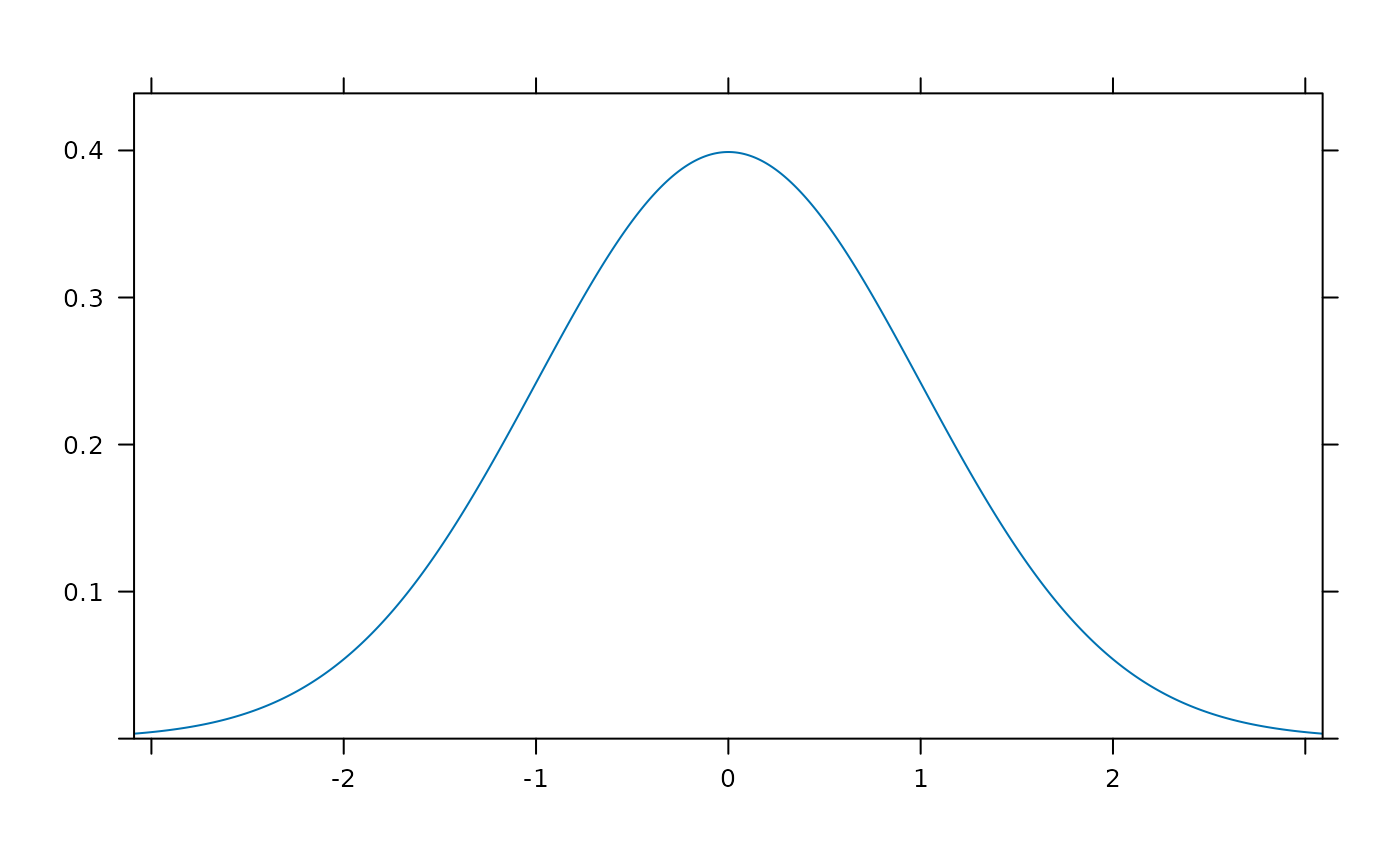
plotDist('norm')

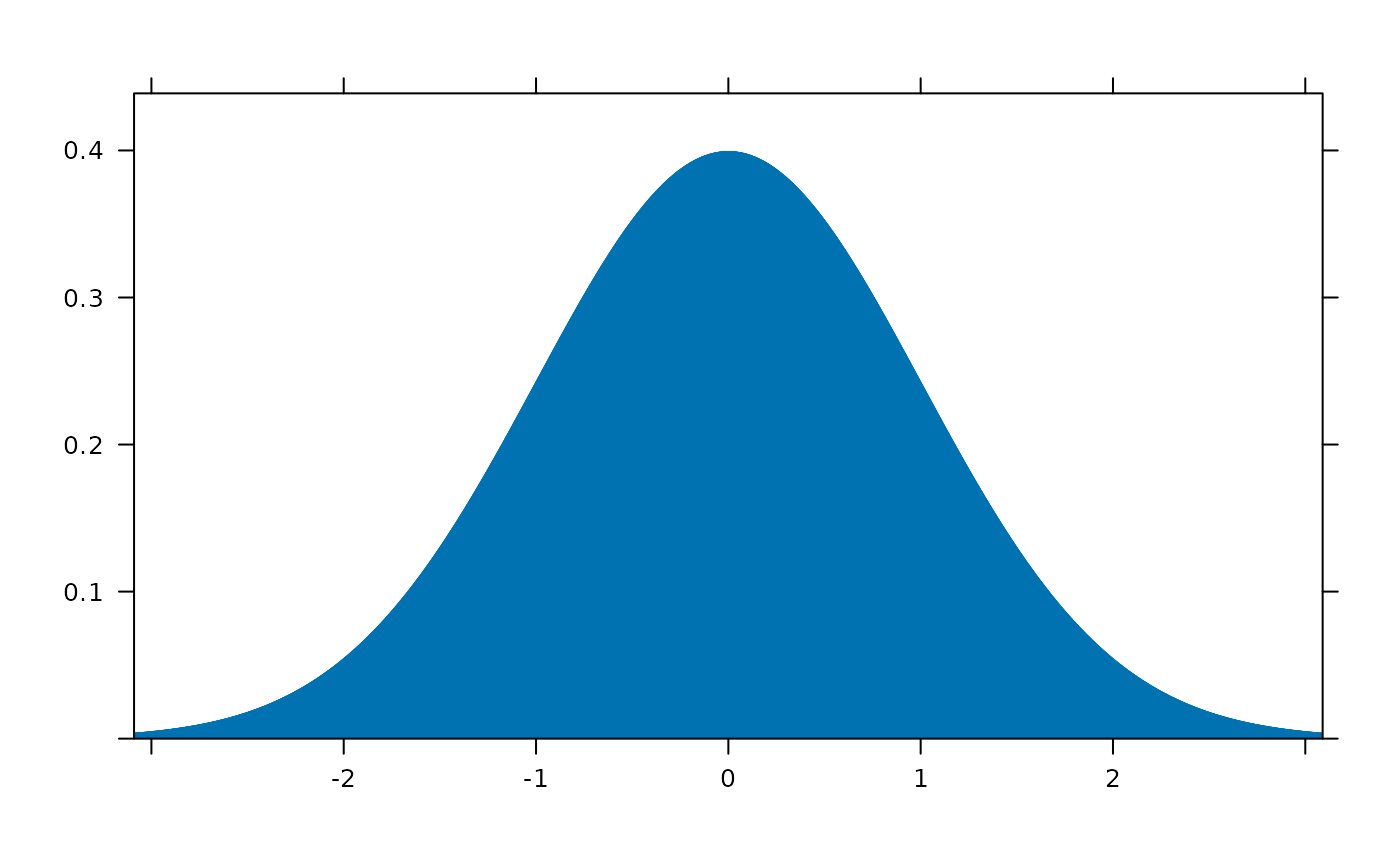
plotDist('norm', type='h')

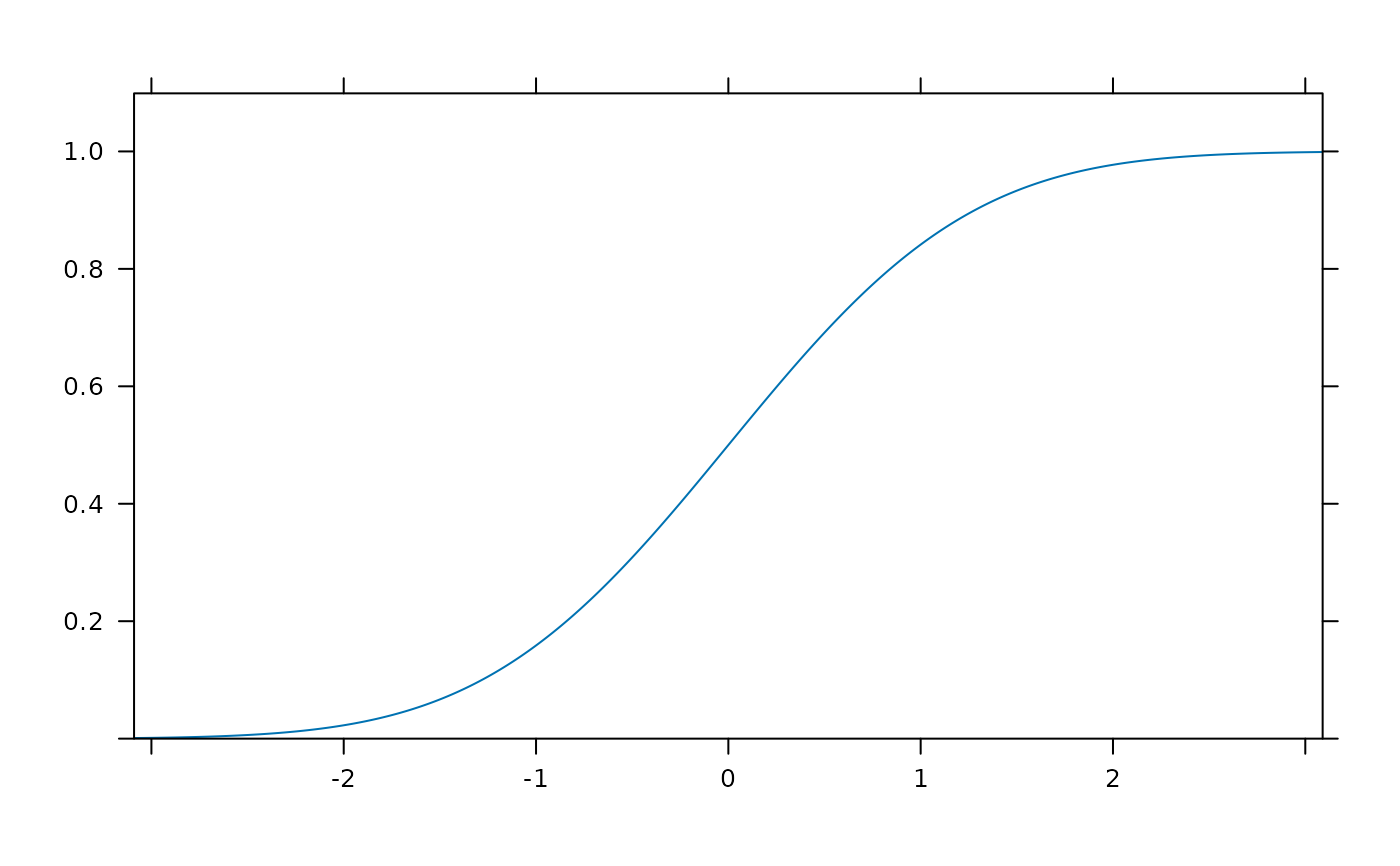
plotDist('norm', kind='cdf')

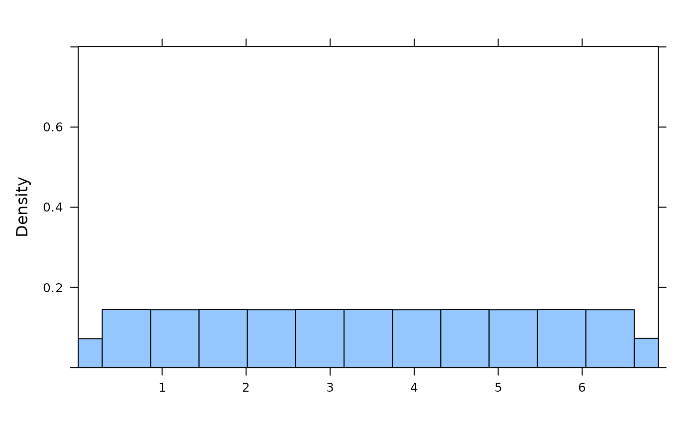
plotDist('exp',  kind='histogram')

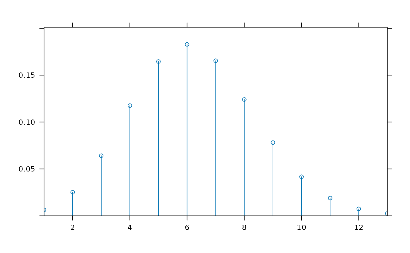
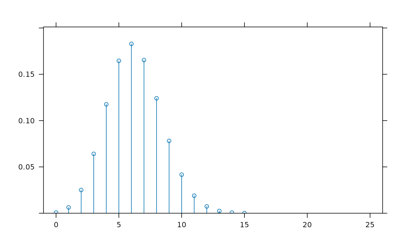
plotDist('binom', params=list( 25, .25))       # explicit params

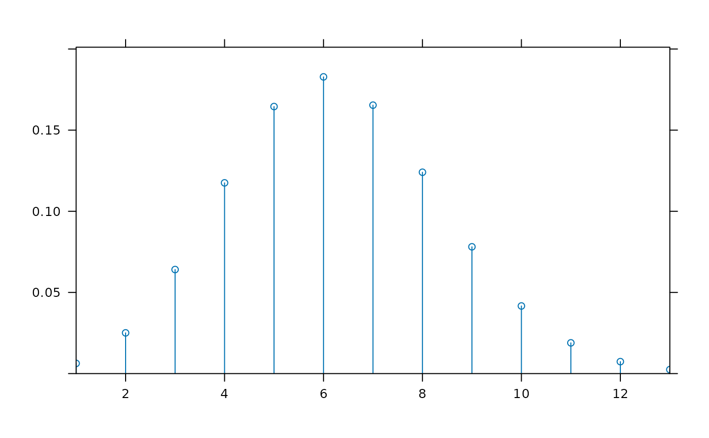plotDist('binom', 25, .25)                     # params inferred

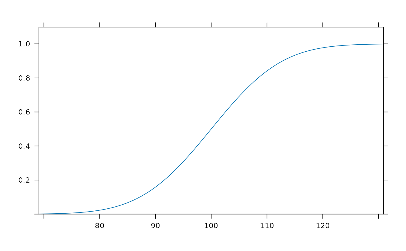
plotDist('norm', mean=100, sd=10, kind='cdf')  # params inferred

plotDist('binom', 25, .25, xlim=c(-1,26) )     # params inferred

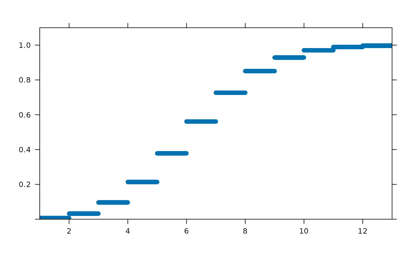
plotDist('binom', params=list( 25, .25), kind='cdf')

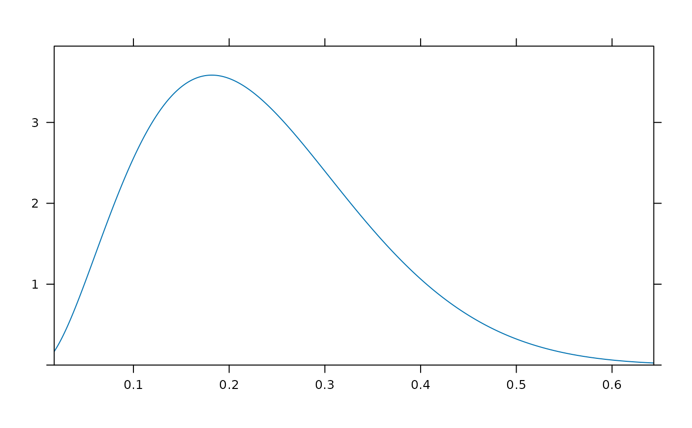
plotDist('beta', params=list( 3, 10), kind='density')

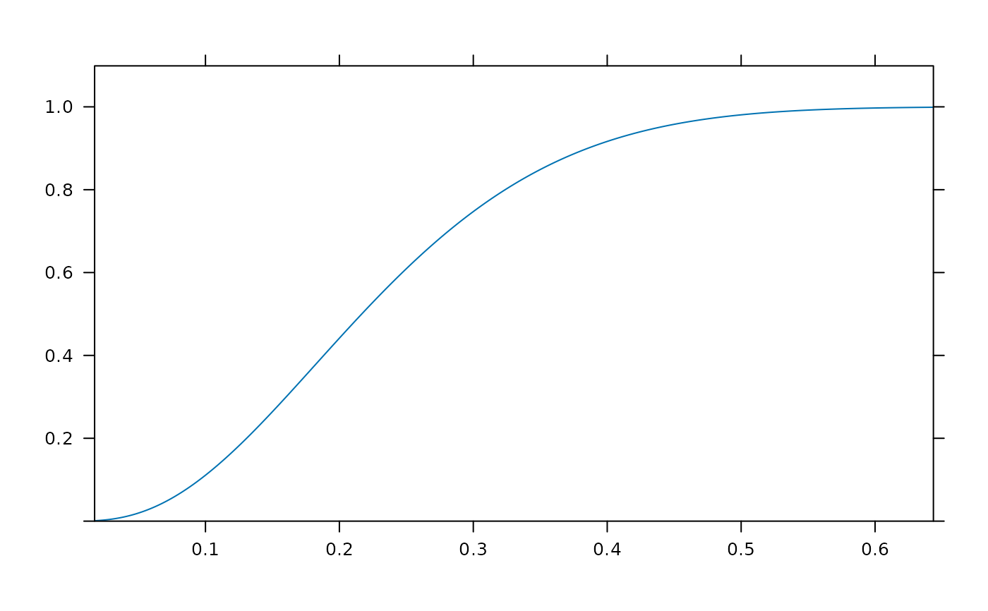
plotDist('beta', params=list( 3, 10), kind='cdf')

plotDist( "binom", params=list(35,.25), 
           groups= y < dbinom(qbinom(0.05, 35, .25), 35,.25) )

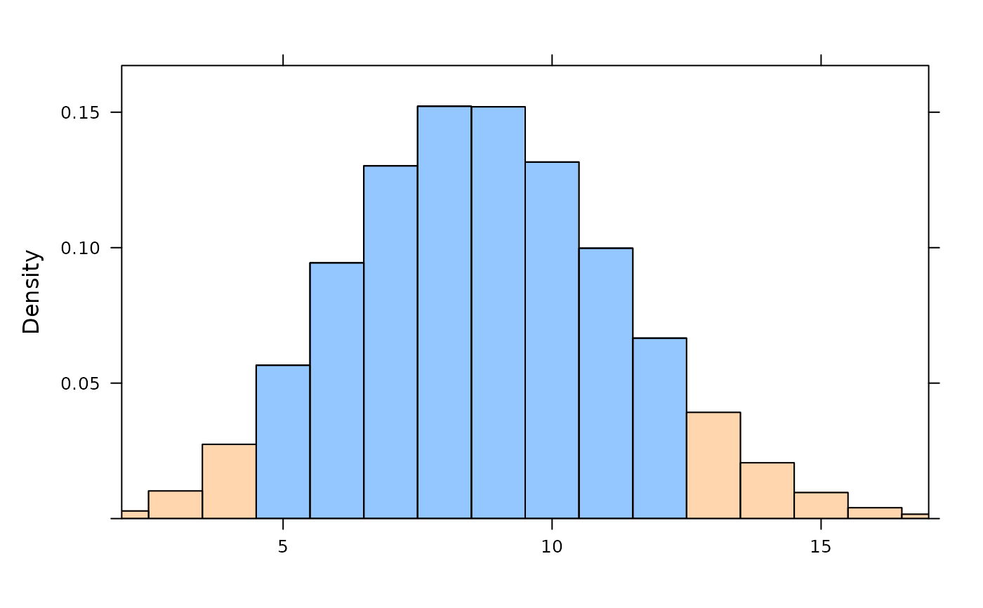
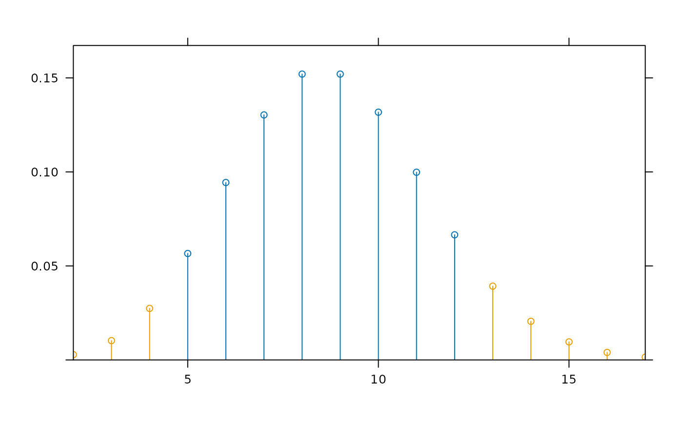plotDist( "binom", params=list(35,.25), 
           groups= y < dbinom(qbinom(0.05, 35, .25), 35,.25), 
           kind='hist')

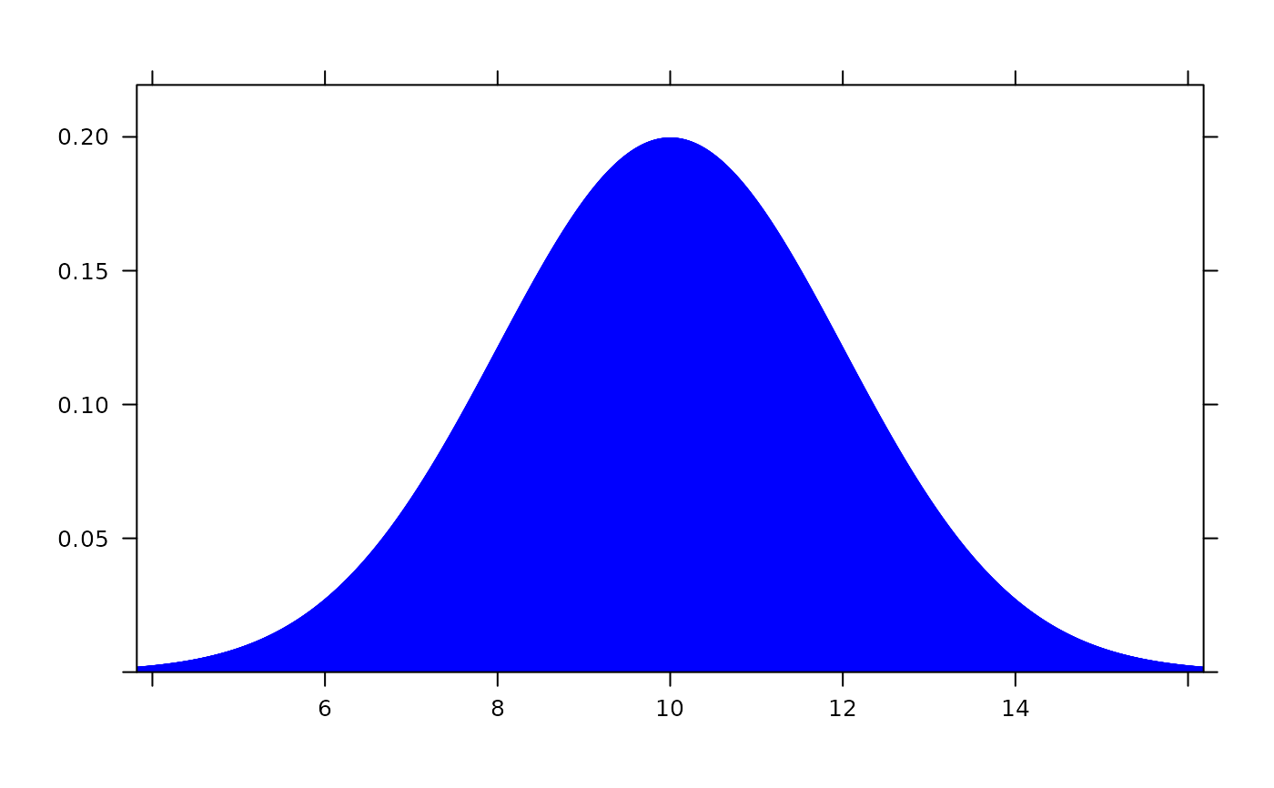
plotDist("norm", mean=10, sd=2, col="blue", type="h")

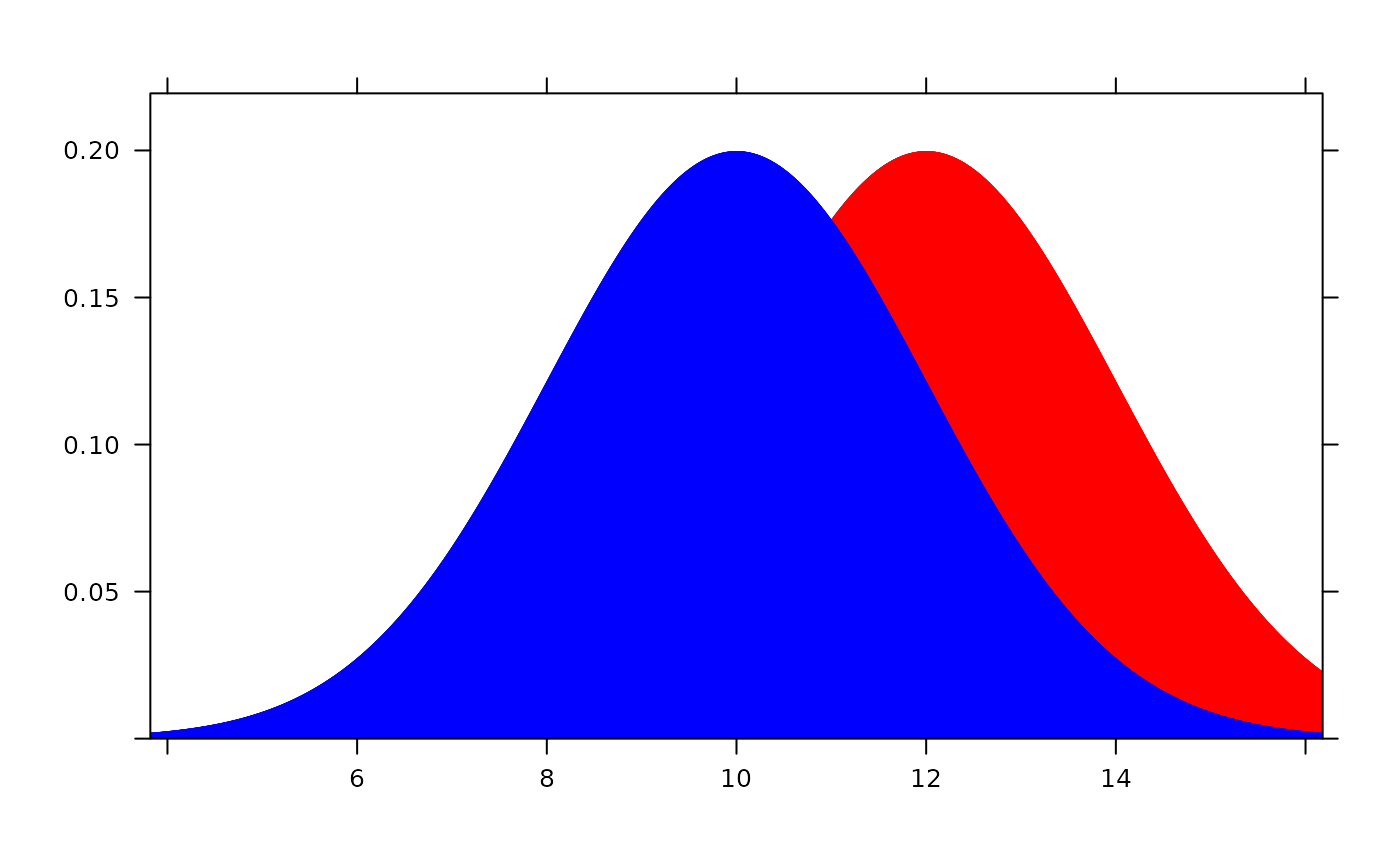
plotDist("norm", mean=12, sd=2, col="red", type="h", under=TRUE)

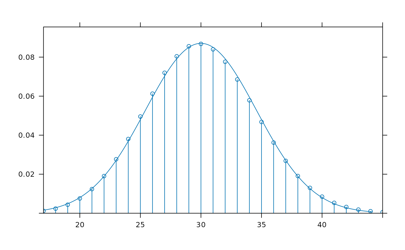
plotDist("binom", size=100, prob=.30) +
  plotDist("norm", mean=30, sd=sqrt(100 * .3 * .7))

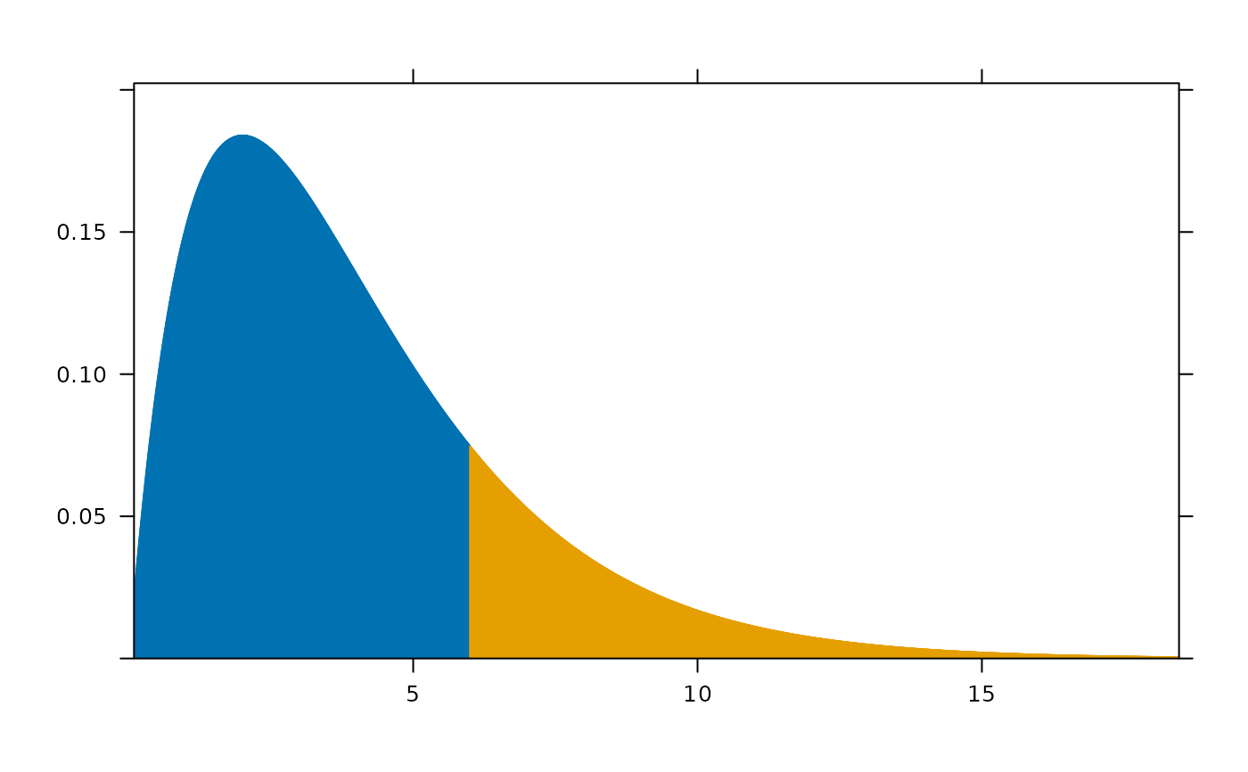
plotDist("chisq", df=4, groups = x > 6, type="h")

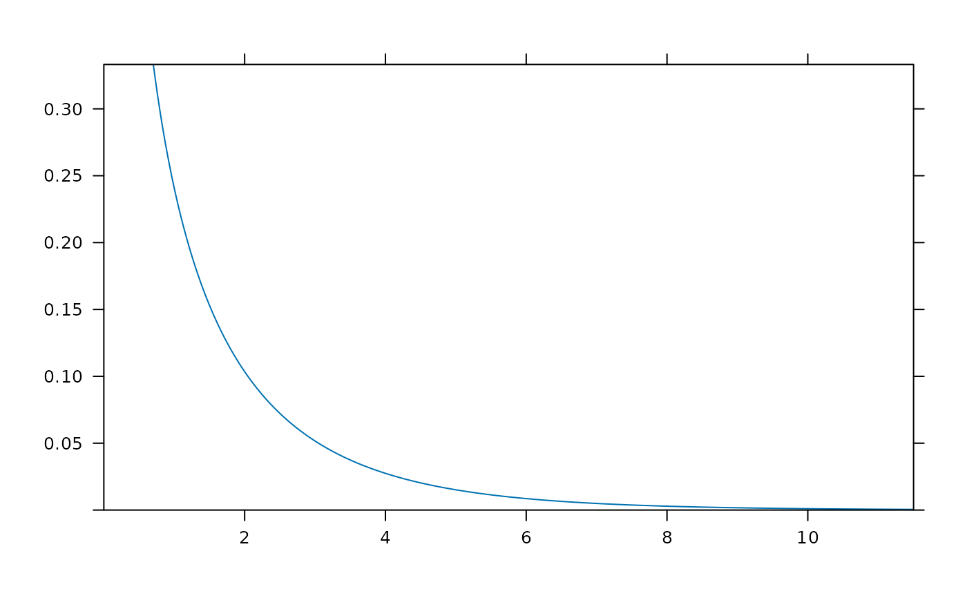
plotDist("f", df1=1, df2 = 99)

if (require(mosaicData)) {
histogram( ~age|sex, data=HELPrct)
m <- mean( ~age|sex, data=HELPrct)
s <- sd(~age|sex, data=HELPrct)
plotDist( "norm", mean=m[1], sd=s[1], col="red", add=TRUE, packets=1)
plotDist( "norm", mean=m[2], sd=s[2], col="blue", under=TRUE, packets=2)
}

Plots of Discrete and Continuous Distributions

Usage

Arguments

Details

See also

Examples