Central portion of a distribution

This function determines the critical values for isolating a central portion of a distribution with a specified probability. This is designed to work especially well for symmetric distributions, but it can be used with any distribution.

Usage

cdist(
  dist = "norm",
  p,
  plot = TRUE,
  verbose = FALSE,
  invisible = FALSE,
  digits = 3L,
  xlim = NULL,
  ylim = NULL,
  resolution = 500L,
  return = c("values", "plot"),
  pattern = c("rings", "stripes"),
  ...,
  refinements = list()
)

xcgamma(
  p,
  shape,
  rate = 1,
  scale = 1/rate,
  lower.tail = TRUE,
  log.p = FALSE,
  ...
)

xct(p, df, ncp, lower.tail = TRUE, log.p = FALSE, ...)

xcchisq(p, df, ncp = 0, lower.tail = TRUE, log.p = FALSE, ...)

xcf(p, df1, df2, lower.tail = TRUE, log.p = FALSE, ...)

xcbinom(p, size, prob, lower.tail = TRUE, log.p = FALSE, ...)

xcpois(p, lambda, lower.tail = TRUE, log.p = FALSE, ...)

xcgeom(p, prob, lower.tail = TRUE, log.p = FALSE, ...)

xcnbinom(p, size, prob, mu, lower.tail = TRUE, log.p = FALSE, ...)

xcbeta(p, shape1, shape2, ncp = 0, lower.tail = TRUE, log.p = FALSE, ...)

Arguments

dist: a character string naming a distribution family (e.g., "norm"). This will work for any family for which the usual d/p/q functions exist.
p: the proportion to be in the central region, with equal proportions in either "tail".
plot: a logical indicating whether a plot should be created
verbose: a logical indicating whether a more verbose output value should be returned.
invisible: a logical
digits: the number of digits desired
xlim: x limits. By default, these are chosen to show the central 99.8\ of the distribution.
ylim: y limits
resolution: number of points used for detecting discreteness and generating plots. The default value of 5000 should work well except for discrete distributions that have many distinct values, especially if these values are not evenly spaced.
return: If "plot", return a plot. If "values", return a vector of numerical values.
pattern: One of "stripes" or "rings". In the latter case, pairs of regions (from the outside to the inside) are grouped together for coloring and probability calculation.
...: additional arguments passed to the distribution functions. Typically these specify the parameters of the particular distribution desired. See the examples.
refinements: A list of refinements to the plot. See ggformula::gf_refine().
shape, scale: shape and scale parameters. Must be positive, scale strictly.
rate: an alternative way to specify the scale.
lower.tail: logical; if TRUE (default), probabilities are \(P[X < x]\), otherwise, \(P[X \ge x]\) (exceptionally not cadlag here, to ensure, e.g., pgamma(0, shape=0) remains zero).
log.p: A logical indicating whether probabilities should be returned on the log scale.
df: degrees of freedom (\(> 0\), maybe non-integer). df = Inf is allowed.
ncp: non-centrality parameter \(\delta\); currently except for rt(), accurate only for abs(ncp) <= 37.62. If omitted, use the central \(t\) distribution.
df1, df2: degrees of freedom. Inf is allowed.
size: number of trials (zero or more).
prob: probability of success on each trial.
lambda: vector of (non-negative) means.
mu: alternative parametrization via mean: see ‘Details’.
shape1, shape2: non-negative parameters of the Beta distribution.

Value

a pair of numbers indicating the upper and lower bounds, unless verbose is TRUE, in which case a 1-row data frame is returned containing these bounds, the central probability, the tail probabilities, and the name of the distribution.

Note

This function is still experimental and changes the input or output formats are possible in future versions of the package.

Examples

cdist( "norm", .95)

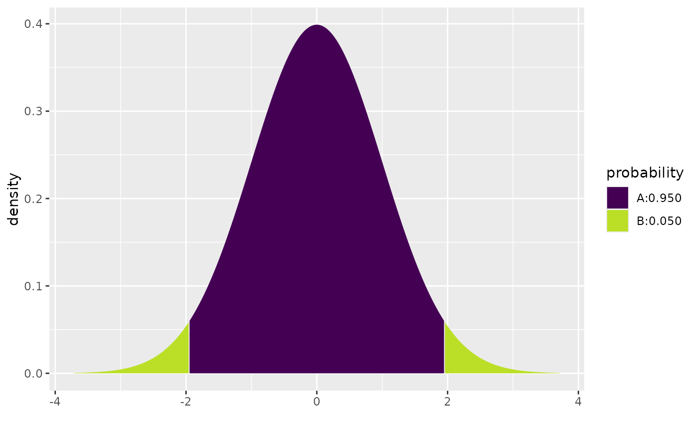#> [1] -1.959964  1.959964
cdist( "t", c(.90, .95, .99), df=5)

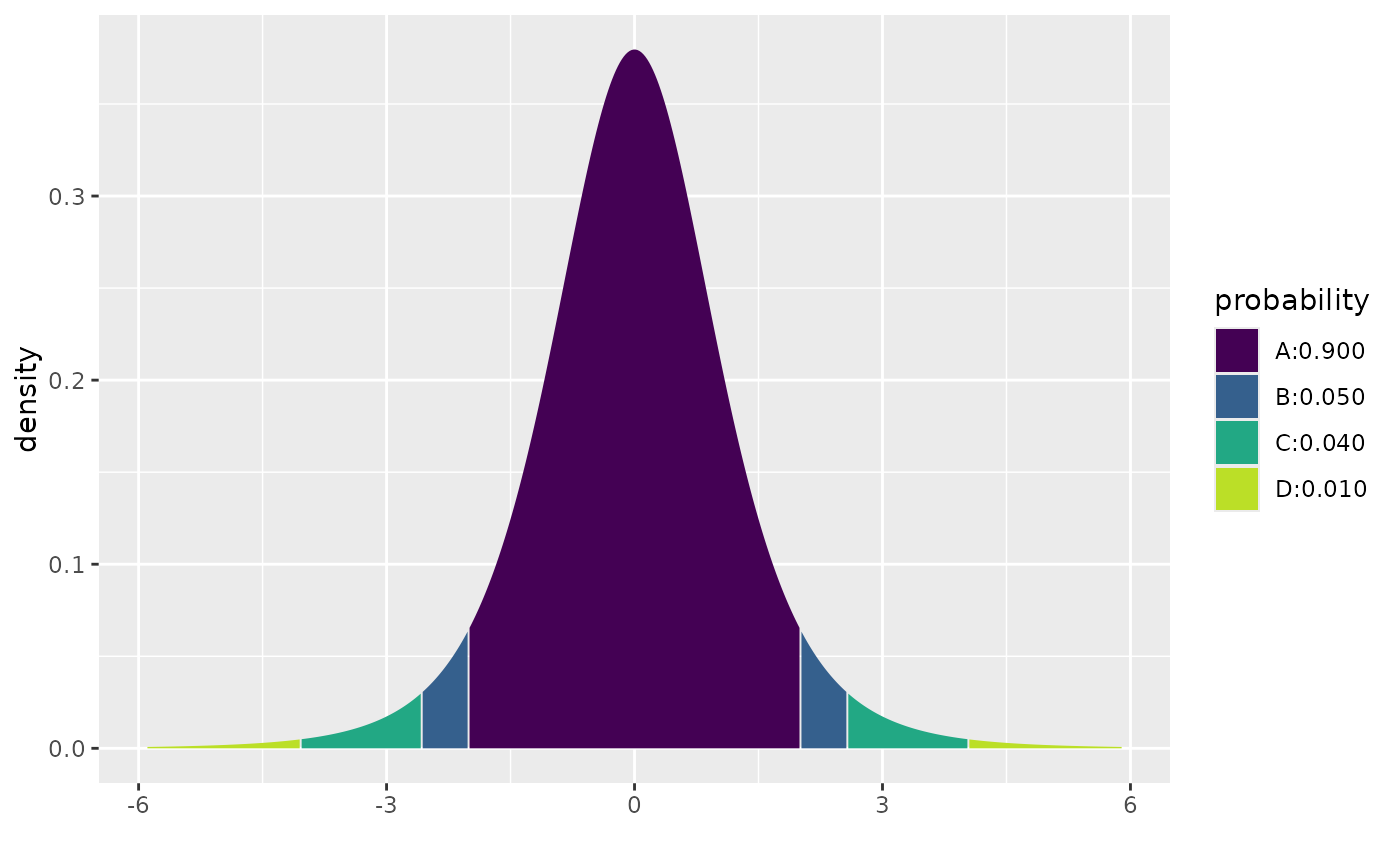#> [1] -4.032143 -2.570582 -2.015048  2.015048  2.570582  4.032143
cdist( "t", c(.90, .95, .99), df=50)

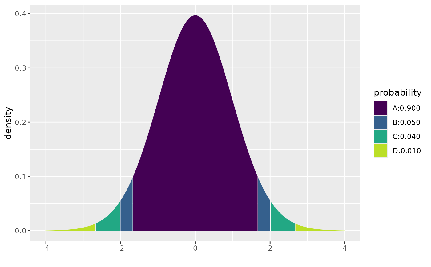#> [1] -2.677793 -2.008559 -1.675905  1.675905  2.008559  2.677793
# plotting doesn't work well when the parameters are not constant
cdist( "t", .95, df=c(3,5,10,20), plot = FALSE)
#>           [,1]     [,2]
#> [1,] -3.182446 3.182446
#> [2,] -2.570582 2.570582
#> [3,] -2.228139 2.228139
#> [4,] -2.085963 2.085963
cdist( "norm", .95, mean=500, sd=100 )

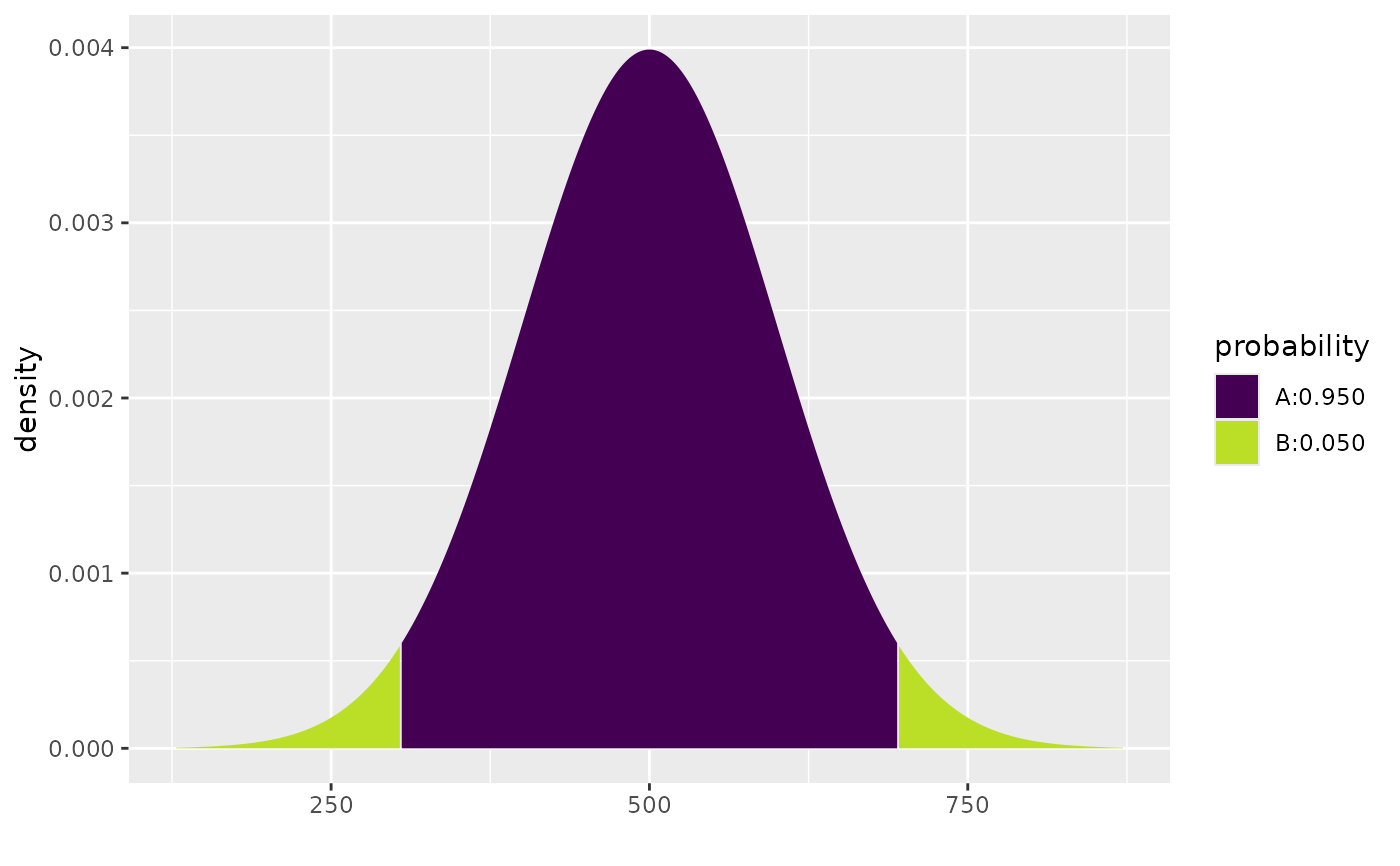#> [1] 304.0036 695.9964
cdist( "chisq", c(.90, .95), df=3 )

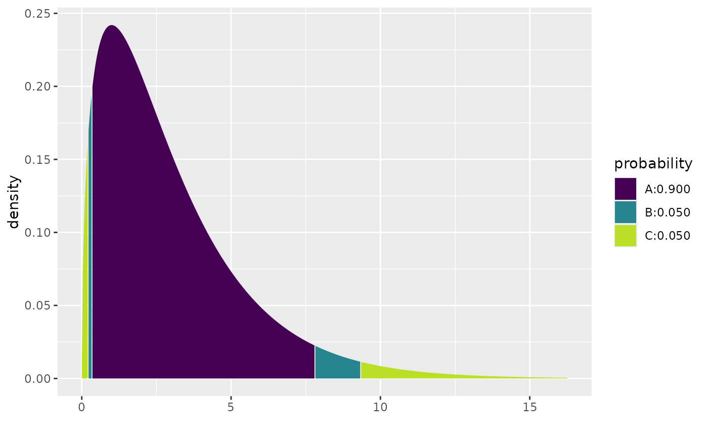#> [1] 0.2157953 0.3518463 7.8147279 9.3484036
# CI
x <- rnorm(23, mean = 10, sd = 2)
cdist("t", p = 0.95, df=22)

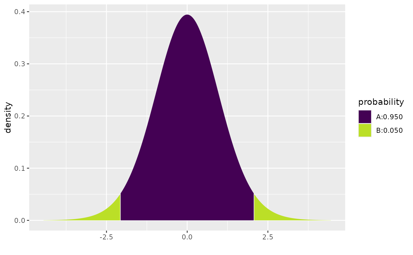#> [1] -2.073873  2.073873
mean(x) + cdist("t", p = 0.95, df=22) * sd(x) / sqrt(23)

#> [1]  9.806628 10.835914
confint(t.test(x))
#>   mean of x    lower    upper level
#> 1  10.32127 9.806628 10.83591  0.95
cdist("t", p = 0.95, df=22, verbose = TRUE)
#> Verbose output not yet implemented.

#> [1] -2.073873  2.073873