The multivariate truncated normal distribution

The probability density function, the distribution function and random number generation for the d-dimensional truncated normal (Gaussian) random variable.

dmtruncnorm(x, mean, varcov, lower, upper, log = FALSE, ...)
pmtruncnorm(x, mean, varcov, lower, upper, ...)
rmtruncnorm(n, mean, varcov, lower, upper, start, burnin=5, thinning=1)

Arguments

x: either a vector of length d or a matrix with d columns,representing the coordinates of the point(s) where the density must be evaluated. Here we denote d=ncol(varcov); see ‘Details’ for restrictions.
mean: a d-vector representing the mean value of the pre-truncation normal distribution.
varcov: a symmetric positive definite matrix with dimensions (d,d) representing the variance matrix of the pre-truncation normal distribution.
lower: a d-vector representing the lower truncation values of the component variables; -Inf values are allowed. If missing, it is set equal to rep(-Inf, d).
upper: a d-vector representing the upper truncation values of the component variables; Inf values are allowed. If missing, it is set equal to rep(Inf, d).
log: a logical value (default value is FALSE); if TRUE, the logarithm of the density is computed.
...: arguments passed to sadmvn, among maxpts, abseps, releps.
n: the number of (pseudo) random vectors to be generated.
start: an optional vector of initial values; see ‘Details’.
burnin: the number of burnin iterations of the Gibbs sampler (default: 5); see ‘Details’.
thinning: a positive integer representing the thinning factor of the internally generated Gibbs sequence (default: 1); see ‘Details’.

Details

For dmtruncnorm and pmtruncnorm, the dimension d cannot exceed 20. If this threshold is exceeded, NAs are returned. The constraint originates from the underlying function sadmvn.

If d>1, rmtruncnorm uses a Gibbs sampling scheme as described by Breslaw (1994) and by Kotecha & Djurić (1999), Detailed algebraic expressions are provided by Wilhelm (2022). After some initial settings in R, the core iteration is performed by a compiled FORTRAN 77 subroutine, for numerical efficiency.

If the start vector is not supplied, the mean value of the truncated distribution is used. This choice should provide a good starting point for the Gibbs iteration, which explains why the default value for the burnin stage is so small. Since successive random vectors generated by a Gibbs sampler are not independent, which can be a problem in certain applications. This dependence is typically ameliorated by generating a larger-than-required number of random vectors, followed by a ‘thinning’ stage; this can be obtained by setting the thinning argument larger that 1. The overall number of generated points is burnin+n*thinning, and the returned object is formed by those with index in burnin+(1:n)*thinning.

If d=1, the values are sampled using a non-iterative procedure, essentially as in equation (4) of Breslaw (1994), except that in this case the mean and the variance do not refer to a conditional distribution, but are the arguments supplied in the calling statement.

Value

dmtruncnorm and pmtruncnorm return a numeric vector; rmtruncnorm returns a matrix, unless either n=1 or d=1, in which case it returns a vector.

Author

Adelchi Azzalini

References

Breslaw, J.A. (1994) Random sampling from a truncated multivariate normal distribution. Appl. Math. Lett. vol.7, pp.1-6.

Kotecha, J.H. and Djurić, P.M. (1999). Gibbs sampling approach for generation of truncated multivariate Gaussian random variables. In ICASSP'99: Proceedings of IEEE International Conference on Acoustics, Speech, and Signal Processing, vol.3, pp.1757-1760. doi:10.1109/ICASSP.1999.756335 .

Wilhelm, S. (2022). Gibbs sampler for the truncated multivariate normal distribution. Vignette of R package https://cran.r-project.org/package=tmvtnorm, version 1.5.

Examples

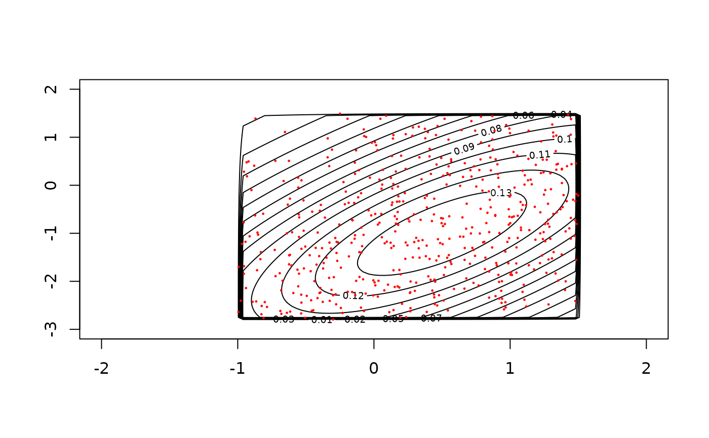
# example with d=2
m2 <- c(0.5, -1)
V2 <- matrix(c(3, 3, 3, 6), 2, 2)
low <- c(-1, -2.8)
up <- c(1.5, 1.5)
# plotting truncated normal density using 'dmtruncnorm' and 'contour' functions 
plot_fxy(dmtruncnorm, xlim=c(-2, 2), ylim=c(-3, 2), mean=m2, varcov=V2, 
      lower=low, upper=up,  npt=101)   
set.seed(1)    
x <-  rmtruncnorm(n=500, mean=m2, varcov=V2, lower=low, upper=up) 
points(x, cex=0.2, col="red")

#------
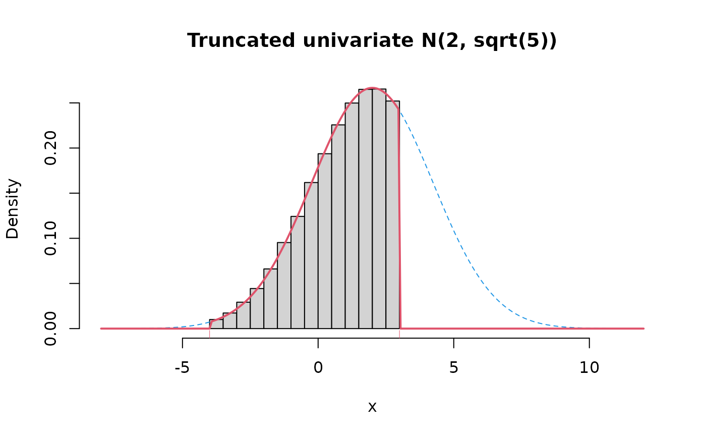
# example with d=1
set.seed(1) 
low <- -4
hi <- 3
x <- rmtruncnorm(1e5, mean=2, varcov=5, lower=low, upper=hi)
hist(x, prob=TRUE, xlim=c(-8, 12), main="Truncated univariate N(2, sqrt(5))")
rug(c(low, hi), col=2)
x0 <- seq(-8, 12, length=251)
pdf <- dnorm(x0, 2, sqrt(5))
p <- pnorm(c(low, hi), 2, sqrt(5))
lines(x0, pdf/diff(p), col=4, lty=2)
lines(x0, dmtruncnorm(x0, 2, 5, low, hi), col=2, lwd=2)