Plotting a function of two variables
plot_fxy.RdPlot a real-valued function f evaluated on a grid of points
of the Cartesian plane, possibly with parameters specified by ....
The type of graphical display can be regulated by selecting the plotting
function among a set of available options.
plot_fxy(f, xlim, ylim, ..., npt=51, grf, grpar)Arguments
- f
either a function or a character string with the name of a real-valued function whose first argument represents the coordinates of points where
fis evaluated; see ‘Details’ for additional information.- xlim
either a vector of abscissae where the
fmust be evaluated, or a length-two vector with the endpoints of such an interval, in which casenpt[1]equally spaced points will be considered.- ylim
either a vector of ordinates where the
fmust be evaluated, or a length-two vector with the endpoints of such an interval, in which casenpt[2]equally spaced points will be considered.- ...
additional parameters to be supplied to
f; these must be named as expected by the specification off.- npt
either an integer value or a two-element integer vector with the number of equally-spaced points, within the endpoints of
xlimandylim, used to set up the grid of points wherefis evaluated; default value:51. When a single value is supplied, this is expanded into a length-2 vector. Iflength(xlim)>2andlength(ylim)>2,nptis ignored.- grf
an optional character string with the name of the function which produces the graphical display, selectable among
"contour", "filled.contour", "persp", "image"of packagegraphics; ifgrfis unset,"contour"is used.- grpar
an optional character string with arguments supplied to the selected
grffunction, with items separated by,as in a regular call.
Details
Function f will be called with the first argument represented by a
two-column matrix, where each row represents a point of the grid on the
Cartesian plane identified by xlim and ylim;
this set of coordinates is stored in matrix pts of the returned list.
If present, arguments supplied as ... are also passed to f.
It is assumed that f accepts this type of call.
The original motivation of plot_fxy was to plot instances of bivariate
probability density functions specified by package mnormt,
but it can be used for plotting any function fulfilling the above requirements,
as illustrated by some of the examples below.
Value
an invisible list with the following components:
x | a vector of coordinates on the \(x\) axis |
y | a vector of coordinates on the \(y\) axis |
pts | a matrix of dimension (npt[1]*npt[2],2)
with the coordinates of the evaluation points \((x,y)\) |
f.values | the vector of f values at the pts points. |
See also
Examples
Sigma <- matrix(c(1,1,1,2), 2, 2)
mean <- c(0, -1)
xlim <- c(-3, 5)
ylim <- c(-5, 3)
#
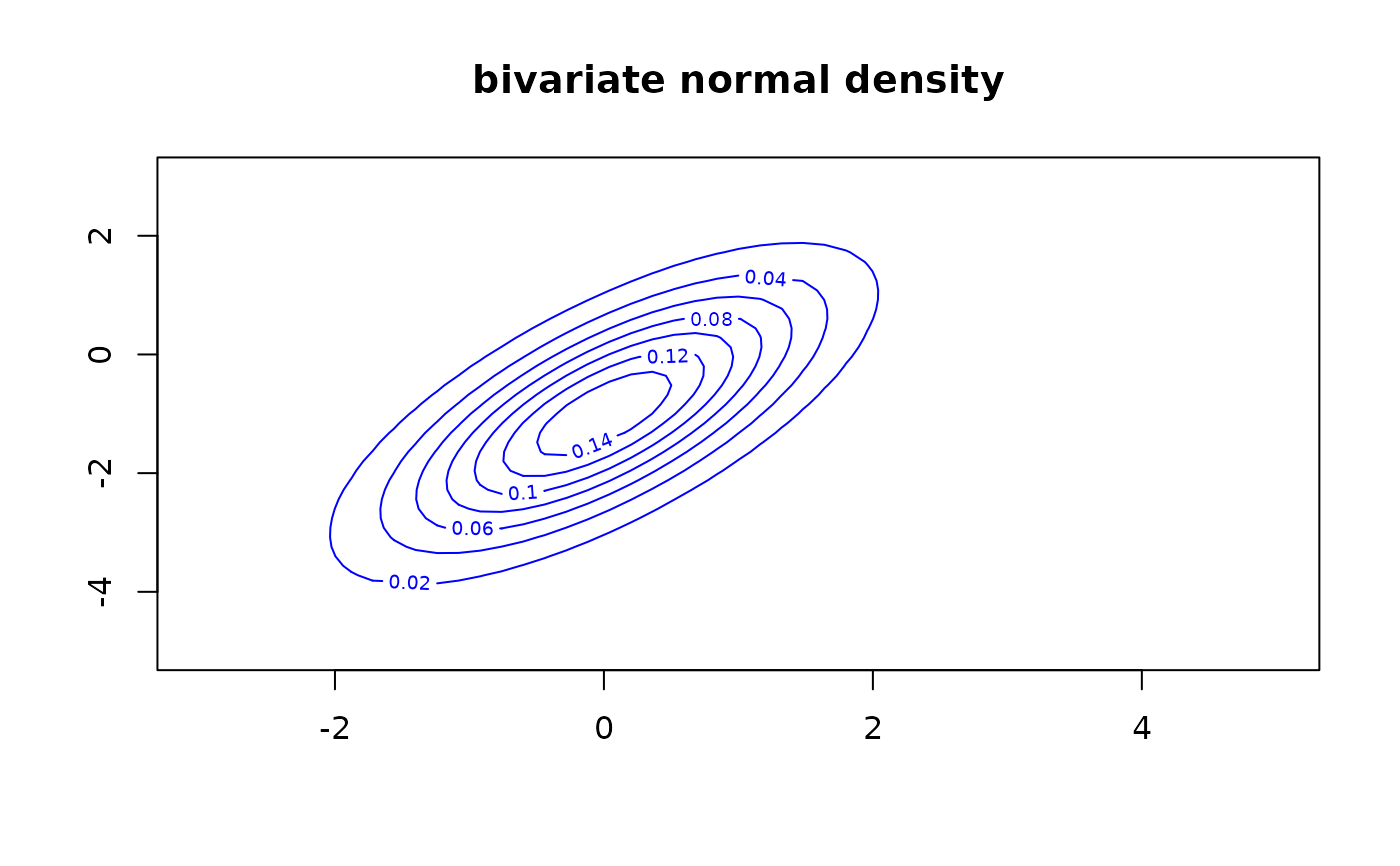
# multivariate normal density, contour-level plot
gp <- 'col="blue", nlevels=6, main="bivariate normal density"'
u <- plot_fxy(dmnorm, xlim, ylim, mean=mean, varcov=Sigma, grpar=gp)
 cat(str(u))
#> List of 4
#> $ x : num [1:51] -3 -2.84 -2.68 -2.52 -2.36 -2.2 -2.04 -1.88 -1.72 -1.56 ...
#> $ y : num [1:51] -5 -4.84 -4.68 -4.52 -4.36 -4.2 -4.04 -3.88 -3.72 -3.56 ...
#> $ pts : num [1:2601, 1:2] -3 -2.84 -2.68 -2.52 -2.36 -2.2 -2.04 -1.88 -1.72 -1.56 ...
#> $ f.values: num [1:51, 1:51] 0.00107 0.00144 0.00184 0.00222 0.00256 ...
#---
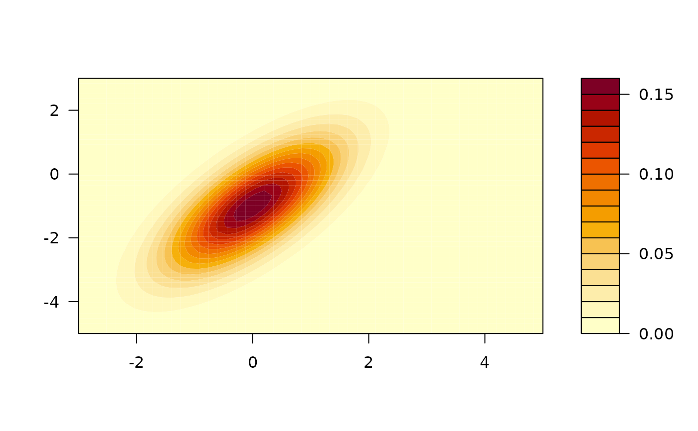
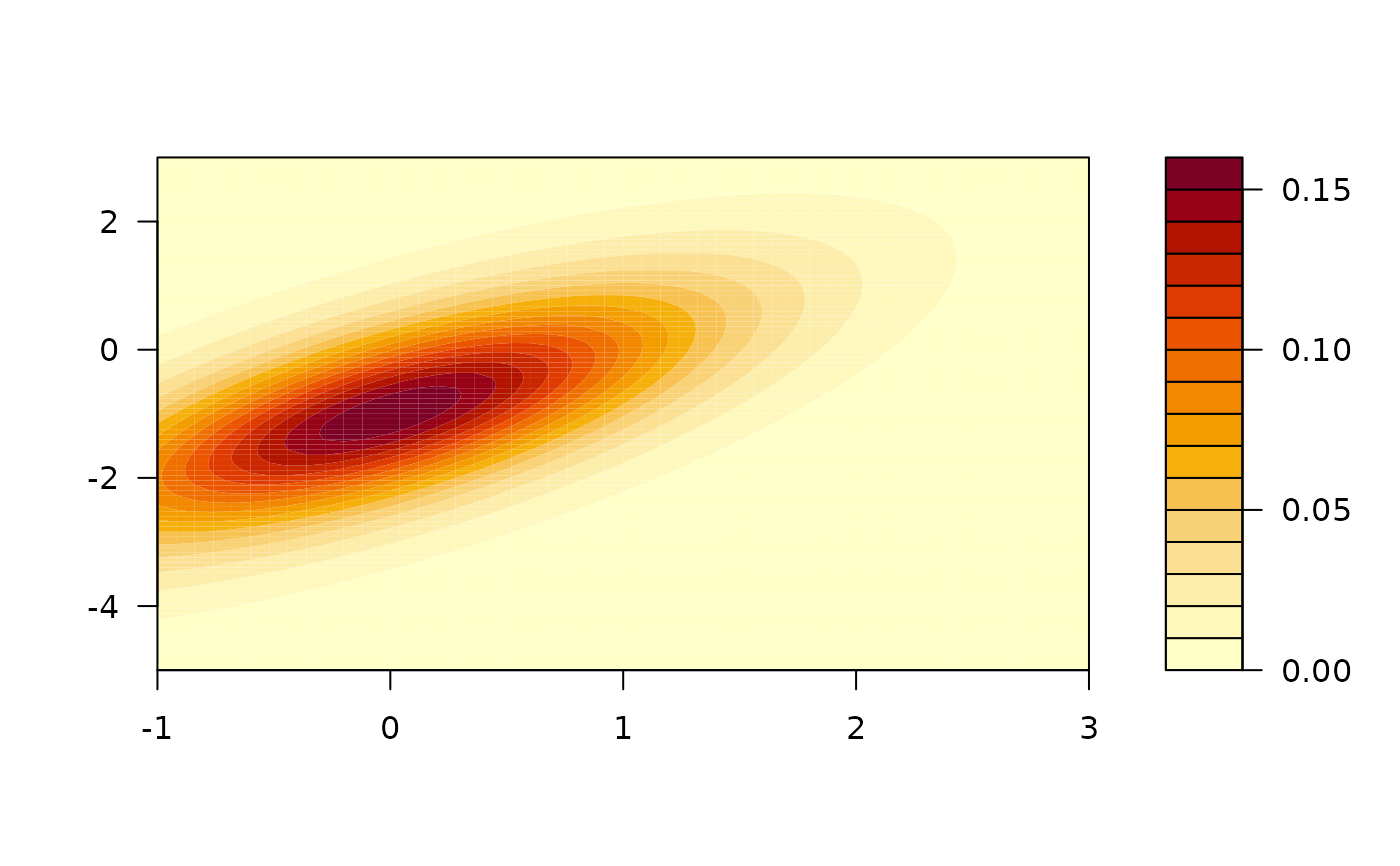
# multivariate normal density, filled-contour plot
plot_fxy(dmnorm, xlim, ylim, mean=mean, varcov=Sigma,grf="filled.contour")
cat(str(u))
#> List of 4
#> $ x : num [1:51] -3 -2.84 -2.68 -2.52 -2.36 -2.2 -2.04 -1.88 -1.72 -1.56 ...
#> $ y : num [1:51] -5 -4.84 -4.68 -4.52 -4.36 -4.2 -4.04 -3.88 -3.72 -3.56 ...
#> $ pts : num [1:2601, 1:2] -3 -2.84 -2.68 -2.52 -2.36 -2.2 -2.04 -1.88 -1.72 -1.56 ...
#> $ f.values: num [1:51, 1:51] 0.00107 0.00144 0.00184 0.00222 0.00256 ...
#---
# multivariate normal density, filled-contour plot
plot_fxy(dmnorm, xlim, ylim, mean=mean, varcov=Sigma,grf="filled.contour")
 #---
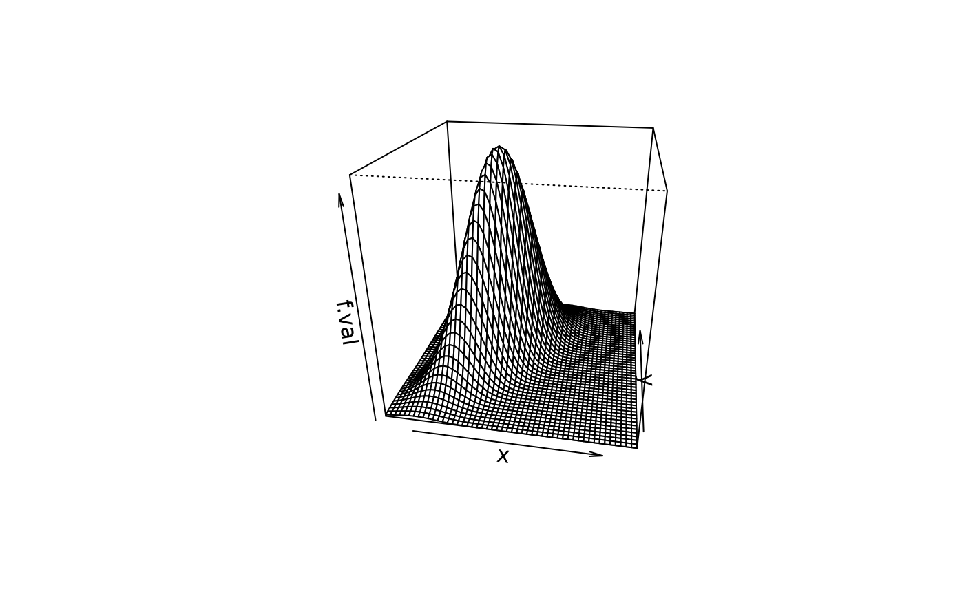
# multivariate normal density, perspective plot
gp <- "theta = 10, phi = 25, r = 2.5"
plot_fxy(dmnorm, xlim, ylim, mean=mean, varcov=Sigma, grf="persp", grpar=gp)
#---
# multivariate normal density, perspective plot
gp <- "theta = 10, phi = 25, r = 2.5"
plot_fxy(dmnorm, xlim, ylim, mean=mean, varcov=Sigma, grf="persp", grpar=gp)
 #---
# multivariate Student's "t" density;
# the xlim argument passed to function 'grf' overrides the earlier xlim;
# xlim and ylim can be placed after the arguments of 'f', if one prefers so
grp <- 'xlim=c(-1, 3)'
plot_fxy(dmt, mean=mean, S=Sigma, df=8, xlim, ylim, npt=101,
grf="filled.contour", grpar=grp)
#---
# multivariate Student's "t" density;
# the xlim argument passed to function 'grf' overrides the earlier xlim;
# xlim and ylim can be placed after the arguments of 'f', if one prefers so
grp <- 'xlim=c(-1, 3)'
plot_fxy(dmt, mean=mean, S=Sigma, df=8, xlim, ylim, npt=101,
grf="filled.contour", grpar=grp)
 #---
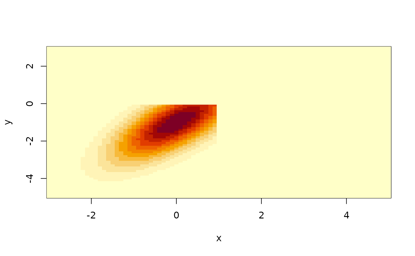
# multivariate truncated normal density, 'image' plot
low <- c(-3, -5)
hi <- c(1, 0)
plot_fxy(dmtruncnorm, mean=mean, varcov=Sigma, lower=low, upper=hi,
xlim, ylim, npt=81, grf="image")
#---
# multivariate truncated normal density, 'image' plot
low <- c(-3, -5)
hi <- c(1, 0)
plot_fxy(dmtruncnorm, mean=mean, varcov=Sigma, lower=low, upper=hi,
xlim, ylim, npt=81, grf="image")
 #---
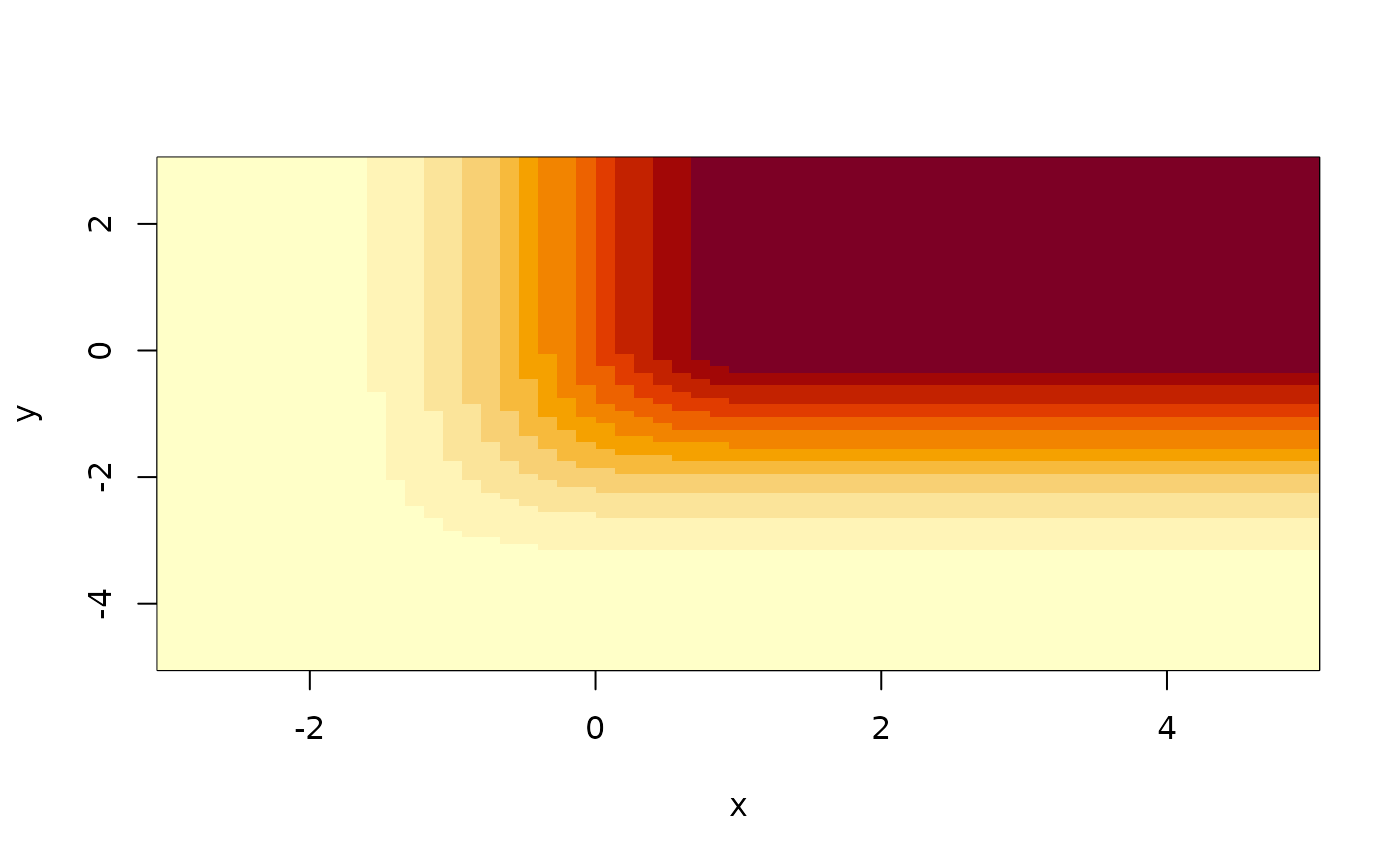
# multivariate truncated normal distribution function, 'image' plot;
# hence not a density function
low <- c(-3, -5)
hi <- c(1, 0)
v <- plot_fxy(pmtruncnorm, mean=mean, varcov=Sigma, lower=low, upper=hi,
xlim, ylim, npt=c(61, 81), grf="image")
#---
# multivariate truncated normal distribution function, 'image' plot;
# hence not a density function
low <- c(-3, -5)
hi <- c(1, 0)
v <- plot_fxy(pmtruncnorm, mean=mean, varcov=Sigma, lower=low, upper=hi,
xlim, ylim, npt=c(61, 81), grf="image")
 #---
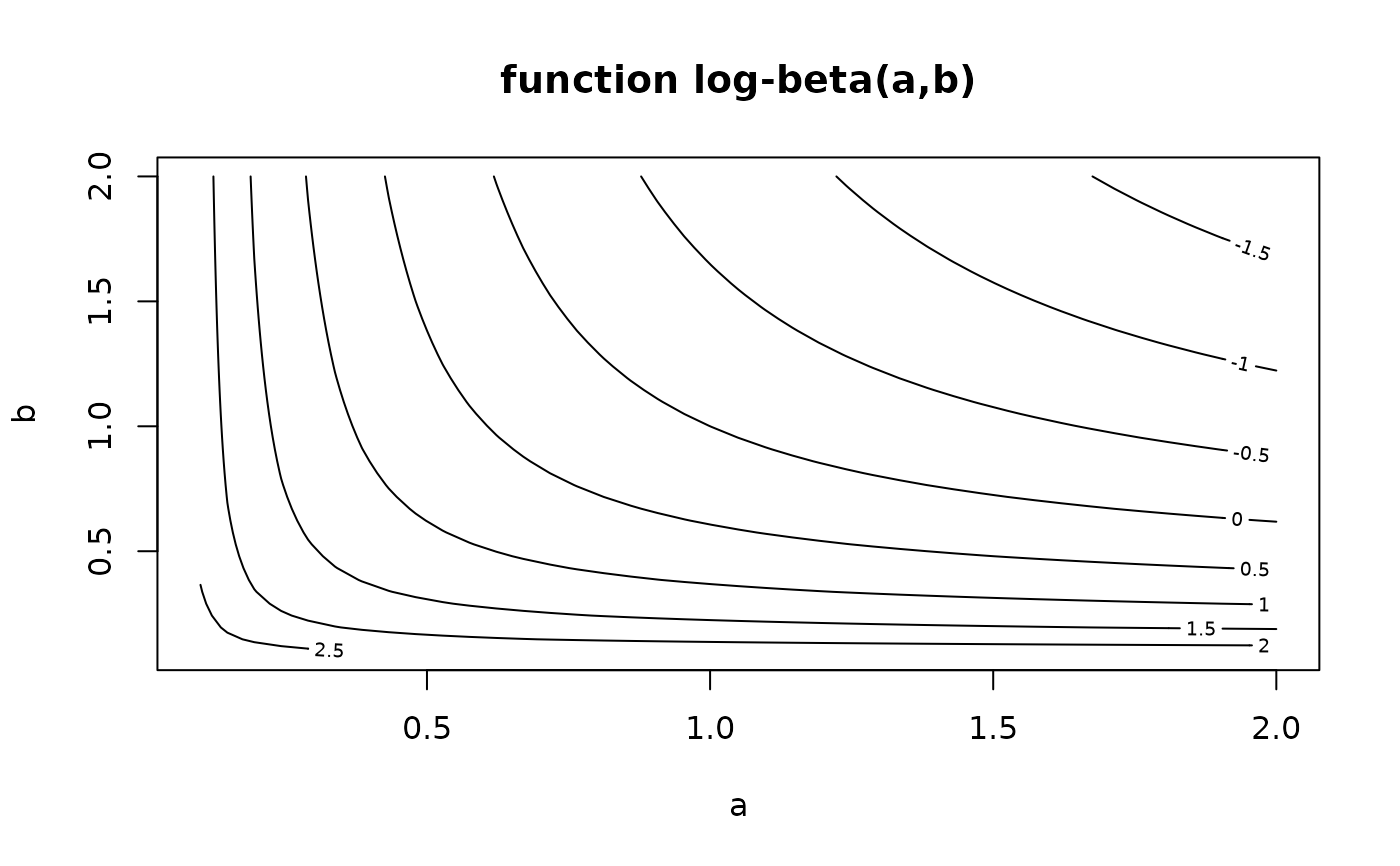
# a different sort of 'f' function (lbeta), not a component of this package
funct <- function(z) lbeta(a=z[,1], b=z[,2])
plot_fxy(funct, xlim=c(0.1, 2), ylim=c(0.1, 2), npt=41,
grpar='main="function log-beta(a,b)", xlab="a", ylab="b"')
#---
# a different sort of 'f' function (lbeta), not a component of this package
funct <- function(z) lbeta(a=z[,1], b=z[,2])
plot_fxy(funct, xlim=c(0.1, 2), ylim=c(0.1, 2), npt=41,
grpar='main="function log-beta(a,b)", xlab="a", ylab="b"')